|
|
|
Abstract
This paper analyses the financial sustainability of the Croatian pension system after the reform that was adopted on January 1, 2019. The Croatian pension system as we know it today was started in 1999 with a reform that created the three pillars of the pension system. Over the next twenty years, Croatian economic and social conditions shifted in an unexpected way and a new reform was needed to ensure financial stability is maintained. In this paper I will analyse population trends in Croatia and forecast movements up to 2060. Afterwards, I will analyse the net government cash flow generated from the pension system, by using the forecast population numbers. The beginning year of the forecast horizon is 2018, as some data were not yet available for this year. I use stochastic methods to perform my analysis.
Keywords: demographic; labour economics; government; Leslie matrix; stochastics forecast; pension system; Croatia
JEL: J11, J13, J14, H55, H68
1 History of the Croatian pension system
The pension system of a country is a necessity for the security of the elderly. It is important for a country to establish and develop a sustainable pension system because it affects all citizens. Such a system can be mandatory or voluntary. Mandatory pension systems are currently widespread, and it is important for citizens to understand how they function and what their individual rights are, since they will be spending their entire lives in the system of their country. We differentiate two types of mandatory pension systems: (1) Defined-Benefit plan and (2) Defined-Contribution plan. A Defined-Benefit (DB) plan promises the individual that they will receive a specific pension amount that depends on the tenure of service and the salary earned. In the DB plan, individuals pay monthly instalments into the pension system. In the Defined-Contribution (DC) plan, individuals are required to put a predetermined amount or percentage of their salary into the “pool” of savings (pension funds). The capital is then invested in different assets and financial instruments, the accumulated capital being afterwards distributed to the individuals once they fulfil the requirements for disbursements. Some countries use the DB plan, others use the DC plan, and some countries use a mixture of both (Puljiz,  2007). 2007).
According to the Croatian Pension Insurance Institute (Mirovinsko.hr, 1999), the Croatian pension system as we know it today was started by the 1999 reform. This was the biggest reform in the pension system since Croatia gained independence. In 1999, three pillars of the pension system were established. The first pillar is mandatory, and it amounts to 15% of the gross salary. This money, which is taken from the employed, is used to provide already existing pensioners with pensions. It is also known as the “pay-as-you-go” pension system (PAYG). The second pillar amounts to 5% of the gross salary, and it can be interpreted as a DC plan, in which the individual’s money is invested in a pension fund in order to gain capital accumulation. As part of the second pillar, individuals may examine the state of their savings at any time. According to the Croatian Financial Services Supervisory Agency (HANFA, 2019), the second pillar is slightly more flexible than the first pillar. Furthermore, individuals can decide to save their money in three different fund categories: A, B and C. If individuals, however, do not personally decide which pension category they want, the authorized institutions will place them in Category B six months after starting their first employment. Each category involves a different amount of risk, and therefore differs depending on the individuals’ rights to invest in different categories of assets and financial instruments. Funds from the Category A are the riskiest ones; Category B is less risky but still riskier than Category C. Category C is known as the safest investment according to the amount of risk. Since the investments in which the money has been placed may decrease in value over time, the country regulates by law the guaranteed amount that will be paid out to each individual once they are eligible for their pension. The third pillar is voluntary, every individual deciding for themselves if they want to save some extra money for old age.
According to the Croatian Pension Insurance Institute (Mirovinsko.hr, 1999), when the 1999 pension reform was introduced, the second and third pillar of the pension system were new. Before the 1999 reform, a certain percentage of individuals’ salary was deducted just in order to pay for the pensions of existing pensioners (PAYG). But after the 1999 reform, 25% of total charges for the pension system were invested in the second pillar – which amounts to 5% of the total salary. The reform started the creation of the second and third pillars on January 1, 2002. Everyone that was aged 39 or less on January 1, 2002, had to accept the two mandatory pillars and 15% (75% of the total contribution amount) of their salary was deducted for the first pillar, and 5% (25% of the total contribution amount) of their salary was deducted for the second pillar. Those that were aged 40 or over on January 1, 2002 were able to decide if they wanted to contribute 20% of their salary to the first pillar or if they wanted to be in the combined pension system. Those individuals that had worked long enough predominantly decided to stay in the first pillar, since the money invested in the second pillar would not be enough in order to offset pensions generated in the first pillar. This was also the case for some people under the age of 40 on January 1, 2002, but they were not given a choice. However, over the next twenty years, many things changed. Croatian demography started shifting in an unexpected way. According to MRMS ( 2019), depending on which pension scheme an individual was using, it was possible for the two individuals, doing the same job and receiving the same salary, to have different amounts of pension just because of the pension scheme they were using. This led to the conclusion that the second pillar was not showing enough strength to offset the pensions that would have been generated if individuals had contributed just to the first pillar. The Croatian government has had increasing cash outflows every year in order to sustain the pension system. Croatia is thus implementing a big new reform of the pension system that started January 1, 2019. The new reform is changing the dynamics of the minimum age to be eligible to receive a pension. Since 2011, the retirement age for the old-age pension, and early retirement, for a woman has been gradually increasing, rising from 60 to 65 by 2030 for the oldage pension and from 55 to 60 for early retirement by 2030 (increasing yearly by 3 months). Starting with 2019, the age limit will be raised by 4 months each year for women, so that by 2027, women and men will retire at the same age. After that, the age limit will be raised by 4 months each year for both sexes until 2033, when individuals will be eligible for retirement at the age of 67 and with 15 years of work experience. The reform includes changes to the early retirement pension, which is also being shifted by four months each year, so that by the year 2033 individuals will be eligible for early retirement at 62 years of age and with 35 years of work experience. Before the 2019 reform, females were eligible for early retirement at 57 years of age and with 32 years of work experience and men at 60 years of age and with 35 years of work experience. The system has been made more flexible; since the 2019 reform, every individual is able to decide upon retirement whether they want to invest their money invested in the second pillar in the first pillar. If they decide to do so, the individual will be considered to have been charged 20% just for the first pillar their entire career. Therefore, everyone can opt for the option that suits them best. According to Mirovinsko.hr ( 2019), the way that the pension is calculated for every individual in Croatia is complex, but an average equation can be worked out. If the individual decides to receive a pension just from the first pillar, the capital accumulated in the second pillar will be sent to the state, and the individual’s pension will be calculated according to equation (1), and an extra 27% will be added to the total (not to all, but only to those with a very low amount of pension). But if the person decides to stay in a combined pension scheme, the pension accumulated by the year 2002 will be calculated by equation (1), and pension accumulated after 2002 will be calculated by the equation (1) and multiplied approximately by 0.75 – since three quarters of the whole pension belongs to the first pillar – and then an extra 20.25% will be added to the calculated result. The rest of the pension will be disbursed from the pension fund, which can be calculated implementing financial mathematics methods. The 20.25% extra, which has been contributed from a combined pension scheme, can be interpreted as a penalty for not investing money in the first pillar. This amount is generated from the second pillar since those who decide to receive their pension just from the first pillar receive an extra 27% of the amount (again, not to all, but only to those with a very low amount of pension) | Pension amount = Personal points * Pension factor * Actual pension value | (1) |
Personal points depend on work experience and wage value through career. The pension factor defines what ratio of personal points will be used in the pension calculation. The value of the pension factor lies between 0 and 1. If the individual fulfils all legal requirements for a pension, his pension factor will be 1. If, however, the individual does not fulfil all legal requirements for going into retirement, they can still retire but the pension factor will be less than 1. The actual pension value is defined by the government – it changes over time in order to reflect the economic state of the country.
In this paper, I will analyse how the pension system might develop in the future by implementing stochastic methods. The idea of implementing stochastic methods in my analysis came from the paper published by Tian and Zhao ( 2016). My whole research includes Walter Enders’ Applied Econometric Time Series ( 2014) as a reference for implementing and analysing time series. First, I will start with an analysis of the population trends. Once future population movements are estimated, the given result will be used in further analysis of government net expenditures for the pension system.
2 Overview of Croatian population trends
The first step in analysing the sustainability of the pension system in Croatia is analysing the country’s demography. A good demographic forecast would solve the problem alone. Therefore, considerable effort will be put into analysing Croatian demography. Firstly, we start with the overall population to get a picture of where are we today. Figure 1 shows the Croatian population trends over the last 18 years.
Figure 1Total population in Croatia (in millions) DISPLAY Figure
A decreasing pattern can clearly be noticed. Over the last 8 years, Croatia’s population has decreased by approximately 200,000. Figure 2 shows Croatian population divided into two age groups, 15-65 and 65+ respectively.
Figure 2Total population in Croatia in two different age groups (in millions) DISPLAY Figure
Here we can see cause for growing concern. While the population of retired citizens is steadily increasing, the population of the working force is swiftly decreasing. After 2011, the population of the working force decreased by approximately 170,000, while the population of people aged 64+ increased by approximately 75,000. This has negatively affected the basic pension system in Croatia. Neither the increasing trend of the population aged 65+ nor the decreasing trend of the population aged 15-64 is showing any signs of stopping. Migration is one of the main drivers of the decreasing trend of working age population. Figure 3 and Figure 4 will try to break down the population movement further.
Figure 3Total population in Croatia in two different age groups (in millions) DISPLAY Figure Figure 4Net migration in Croatia (in thousands) DISPLAY Figure
The population of people aged 20-34 has decreased by approximately 100,000 (110,000 from its peak point), while the population of people aged 35-64 has decreased by approximately 30,000 (70,000 from its peak point). Croatia showed positive net migration up to 2009. Figure 3 shows that this immigration has mostly impacted the numbers of the older age group. From the beginning of 2010, Croatia has had a negative net migration, which is mostly shown in the younger part of the working age population. Therefore, the younger population has had a more significant influence on the decrease in the total working age population. The main reason may be that the young are not satisfied with the economic, social, educational or many other opportunities offered in Croatia, so they try to find better opportunities in other countries. Since July 2013 Croatia has been a member of the EU. Upon the country’s entry, a sharply decreasing trend in net migration occurred. The question is whether the current trend will continue to develop in a similar way. In my opinion, the short-term answer is yes, but the long-term no. In order to answer this question, the Croatian population can be separated into three groups: (1) Those that want to leave Croatia, (2) Those that do not want to leave Croatia, and (3) The undecided. Group (3) can be excluded because its members will eventually migrate to groups (1) or (2). Group (1) consists of a certain amount of the total population which is constant. Once all its members leave the country, the immigration wave will stop. Group (1) is also not leaving the country in the blink of an eye – this trend is dynamic, dependent on time, as well as other variables. Therefore, it will take time until this trend is finished.
3 Introduction to the Leslie Model
The model used in forecasting in this analysis is the Leslie model. The Leslie model is set as follows (Cull, Flahive and Robson, 2005):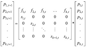 | (2) |
where L= 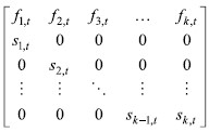 is called the Leslie matrix is called the Leslie matrix |
|
pi,t ~ number of individuals in iTH age group at time t fi,t ~ number of births per individual in iTH age group at time t si,t ~ survival rate in iTH age group at time t.
Variable pi,t is the population in iTH age range. Let us call them cohorts throughout the analysis. There is a total of 18 cohorts in this analysis. The first one is newborns in a given year, the second one is the population aged 1-4, the third one is the population aged 5-9 and so on. The last cohort is the population aged 80+.
It is important to note that parameters f1,t and s1,t are changing over time. If the parameters do not vary over time, the upper equation turns into a matrix difference equation that can be solved as follows: 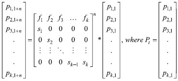 is initial population is initial population |
|
Since the given parameters vary over time, the solution for our equation is as follows:
| (3) |
Vector Pt is the given population at time t, which in our case is 2017. The parameters fi and si are not constant and time series analysis will be implemented in order to estimate the dynamics of the parameters fi,t and si,t. By estimating those parameters, we can estimate the population after n years. In this paper, I will analyse the dynamics of the variables according to the 17 observable data points through time, and then I will implement a stochastic forecast by carrying out 500 Monte Carlo simulations. This method will give us a wider picture of where the population as a system is converging. The changes will be implemented in the Leslie model, which will be described in detail later in the paper.
3.1 Newborns per person
According to the work of Smith, Tayman and Swanson (2013), fertility rates are one of the main variables that affect population growth. Therefore, we will start with analysing fertility rates. We start by analysing the number of births per individual in a iTH age group. This number can be derived from the country’s fertility rates. The fertility rate is the number of children per woman in different age groups. Since we need the data to be the number of newborns per individual, we will transform the data with the following equation: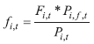 | (4) |
Pi,f,t ~ female population in iTH age group at time t.
The value of fi,t now represents the number of newborns per individual. It would be much better if there were data available on newborns per mother’s age, but these data are rather restricted (just 11 observations are available), so we are forced to use fi,t as calculated by the above formula. The formula itself is a very good proxy compared to the real data of newborns available (the standard deviation on average is approximated to 0.63%).
The first step was forecasting through a time series analysis for each cohort, but I ran into problems of rejecting the random walk hypothesis in the Dickey-Fuller test for some parts of the series. Table 1 shows the results of the Dickey-Fuller test:
Table 1Dickey-Fuller test statistics results for random walk and random walk with a drift DISPLAY Table Table 2Dickey-Fuller statistics and confidence intervals for the data of 16 observations DISPLAY Table
We can now compare the results with 95% confidence intervals given in Table 2. The first model is random walk, and the second model is random walk with drift. To reject the hypothesis that the model is following a random walk process – or random walk with drift – with 95% confidence intervals, the test value must be higher than the absolute value of the Dickey-Fuller test. It can be noticed that this is not the case for all of the series. Therefore, the second approach was used and it yielded much better estimates and results.
3.1.1 Lee-Carter Model for Newborns Per Person
According to Khan, Afrin and Masud ( 2016), the Lee-Carter model is one way to approach the problem of forecasting mortality rates. Here, this method will be used to forecast newborns per person. The model is set as follows: and| log(ƒi,t) = ai + bi * kt + εt | (5) |
where 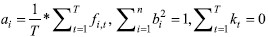 |
|
zi,t = log(fi,t) – ai, where ai are fitted values.
Then we apply singular value decomposition to obtain the product of the three matrices: SVD(Zi,t = U * Λ * VT = Λ1Ui,1Vt,i + ⋯ + ΛnUi,nVt,n. We derive bi from the first row of the age-group component matrix i.e. bi = Ui,1, and kt is derived from multiplication of the time component matrix and the first eigenvalue i.e. kt = Λ1 * Vt,1. Estimated values of ai and bi are shown in Table 3.
Table 3Parameters in the Lee-Carter model DISPLAY Table
Parameters bi reveal a lot about the trend that is present. Parameter bi directly affects newborns per person rates each time when the index kt is changed. It can be seen that the parameter bi has negative values for age groups 15-29 and positive for age groups 30-49. These values show that the number of young people aged 15-29 who are having children is decreasing. Instead, people start having children at the ages of 30-49. This trend is present worldwide, not just in Croatia.
Now we have all the necessary parameters. We now need to forecast the future values of kt. First, we start by checking stationarity. Table 4 shows Dickey-Fuller test statistics:
Table 4Dickey-Fuller statistics for newborns per person index DISPLAY Table
Data from Table 2 can be used for comparison since the number of observations and the value of the confidence intervals is the same. The parameter α1 in the first equation (random walk without drift) is statistically different from zero with 95% confidence, so we reject the hypothesis that this process is random walk with a 95% confidence level. When it comes to the second equation, the confidence level is even higher. We can thus reject the hypothesis that α1 is equal to zero with a 99% confidence level, and that the constant parameter together with α1 is statistically different from zero with a 99% confidence level.
The following two figures, Figure 5 and Figure 6, show the autocorrelation function (ACF) and partial autocorrelation function (PACF) of the newborns per person index. They are used in order to decide which process describes movements in the newborns per person index the best.
Figure 5Autocorrelation function (ACF) for newborns per person index DISPLAY Figure Figure 6Partial autocorrelation function (PACF) for newborns per person index DISPLAY Figure
The autocorrelation function shows that the current kt on average correlates with the previous three observations, but the partial autocorrelation function indicates that the movements in kt are best explained by just one lagged dependent variable. Our conclusion is that the autoregressive model of order 1 (AR (1)) that includes the intercept term will be applied in order to forecast future changes in the newborns per person index. Estimating with ordinary least square approximation, we obtain the results shown in Table 5:
Table 5AR (1) process of newborns per person index DISPLAY Table
The standard error of the lag dependent term is 0.0458, which makes it statistically different from zero with a confidence level of 99%. The standard error of the intercept term is 0.61, which means that it is not statistically different from zero. However, we will include it in the model since the Dickey-Fuller test has demonstrated that that model is better with an intercept term. Now I create 500 simulations by setting equation kt = 0.0528 + 0.9639 * kt–1 + 0,1975 + εt, where εt~Normal(0,1). The results of the simulations are shown in Figure 7.
Figure 7Stochastic simulation results for newborns per person index DISPLAY Figure
Now we have all the necessary data for simulating future values of newborns per person rates for each age group. The following two figures, Figure 8 and Figure 9, are given as final process of stochastic simulations of newborns per person rates for different age groups. We will later use this results in our Leslie matrix.
Figure 8Stochastic simulation results for newborns per person rates, age group: 15-19 DISPLAY Figure Figure 9Stochastic simulation results for newborns per person rates, age group: 30-34 DISPLAY Figure
All those stochastic simulations enable us to generate simulations of total newborns per person rates. We all are much more familiar with the term total fertility rates, meaning the average number of births per mother. Since we are transforming the data to newborns per person rates (not per mother), and the numbers of men and women in Croatia are approximately equal (male population amounted to 49.9% of the total population in 2018), we can therefore by rule of thumb multiply the total newborns per person rates by two in order to get fertility rates. Figure 10 shows total newborns per person rates generated from a stochastic simulation.
Figure 10Stochastic simulation of total newborns per person rates, time horizon: 2017-2060 DISPLAY Figure
In 2017 the total newborns per person rate was 0.7. By multiplying this number by two we receive an approximate fertility rate of 1.40. This is a good approximation if we compare it to the official Eurostat calculation of 1.42. Figure 10 shows forecasted values from 2017 to 2060. It can be seen that most of the data lie at values above 0.7, meaning that this model expects a higher total newborns per person rates in the future. It can be concluded that higher fertility rates are to be expected in the future 1.
3.2 Survival rates
According to Smith, Tayman and Swanson (2013), the next important factor that needs to be estimated for our Leslie matrix is the survival rate si. The survival rate represents the probability that an individual will survive the given age group. To estimate this parameter, we will use the number of deaths in a given age group. The following formula will be used to transform the data: | (6) |
where  |
|
The transformed data now represents the survival rate in each age group at time t. We will again use the Lee-Carter model (Khan, Afrin and Masud, 2016) to simulate future values of number of deaths in each age group.
We set our model as follows: | log(mi,t) = ai + bi *Š kt + εt | (7) |
where 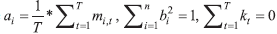 . . |
|
The ai parameter in this equation represents the average age-specific mortality in different age groups. Vector kt is the mortality index that is independent of each age group and varies with time. Each bi parameter shows how change in the mortality index affects mortality rates in different age groups. The same procedure is used as with newborns per person to get correct forecasts of mortality rates. Estimates for ai and bi are given in Table 6.
Table 6Parameters for mortality index in the Lee-Carter model DISPLAY Table
When it comes to parameter kt, a time series analysis will be used first. Checking stationarity, we run into a problem. Table 7 shows Dickey-Fuller test results for the mortality index.
Table 7Dickey-Fuller statistics for mortality index DISPLAY Table
If these results are compared with those in Table 2, the data do not show enough confidence to reject the hypothesis that this process is random walk or random walk with drift with 95% confidence. We can set the model to be pure random walk without drift, and simulate future values, but that is not what I will do. The parameters bi show how the change in kt affects change in mortality rates in a iTH age group. By observing all the negative bi parameters, we expect the value of kt to increase over time. Generally, life expectancy has increased by a large margin over the last 100 years. Many factors affect this, and it is a trend that I expect will continue. The following Figure 11 shows observed values of the mortality index.
Figure 11Mortality index over time DISPLAY Figure
We can notice from Figure 11 that the index shows a trend. I will assume here that this trend is linear. The reason for this assumption is that I do not expect the trend of decreasing patterns of mortality rates to stop. If we set our process to be pure random walk, then the expected future value is also the last observable value, and we lose the trend in the mortality index. An example of the mortality rates in the United States of America (USA) for the age group 15-19 is given in Figure 12.
Figure 12Mortality rates in the USA for the period of 1930-2017 DISPLAY Figure
The example of the United States of America is used in Figure 12 because a large database can be drawn upon. Figure 12 illustrates that the data show a clearly declining trend. The trend shows characteristics of exponential decay. Since our mortality rate values are displayed as logarithms, by displaying the mortality index as a linear trend, we are creating exponential decay for mortality rates. From this assumption follows our new model for mortality index:
kt=β0 + β1 * t + εt, where εt~ random disturbance.
Once we estimate β1 with the ordinary least square estimator, we check the stationarity of the process Kt=kt-β0-β1 * t. Table 8 shows the Dickey-Fuller test results.
Table 8Dickey-Fuller statistics for mortality index set as a model with linear trend DISPLAY Table
The data is stationary, so we can work with it further. The estimated parameters are shown in Table 9.
Table 9Estimated parameters for mortality index DISPLAY Table
The adjusted R2 is 0.95 and the standard deviation of whole model is 0.147. Now we estimate the stochastic model kt = –1.201168 + 0.133463 * t + 0.147 * εt, where εt~Normal(0,1) by doing 500 simulations. Figure 13 shows the results of these mortality index simulations.
Figure 13Mortality index simulations DISPLAY Figure
Now we have all the needed data to simulate mortality rates per cohort. We are now dealing with 18 data sets rather than 7 (as is the case with fertility rates). Figures 14 and 15 are given as examples of simulation results for two different cohorts. We can clearly observe an exponentially decreasing mortality rate trend.
Figure 14Simulated results for mortality rates for the first cohort: newborns DISPLAY Figure Figure 15Simulated results for the mortality index for group aged 45-49 DISPLAY Figure
3.3 Total population
Now we have all the parameters needed for creating our Leslie model. The original Leslie model is set as follows: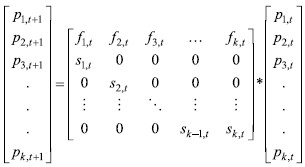
But as I have already mentioned, I will implement some changes in order to produce more precise forecasts. If we use the model as set above, the resulting forecasts will be biased. We need to look at and understand the fundamentals of the model. The output of the model is the population in each cohort. The way that the first cohort is created is a product of matrix multiplication: f1,t * p1,t * … * fk,t * pk,t.The value of fertility rates forecast for a given year is multiplied with that year’s population in order to generate the number of newborns. Then for the next year, the number of new newborns is multiplied with the survival rate of the newborns’ age group, and the value of those who survive is shifted into the next cohort, age group 1-4. For the year after that, the second cohort is multiplied with the second cohort’s survival rate, and the value of those who survive is then shifted into the third cohort, age group 5-9. This is not what actually happens. The population that is aged 1, 2 or 3 remains in the second cohort. The model will be biased if we shift them all into the next cohort. By setting our model in this way, we are shifting the population in each period for five years, and thus generating forecasts for 5 years in each step. But because our fertility and survival rates are set per year, we are in a way dealing with apples and pears. We need to set the model in a such way that it shifts only the oldest members of a given population in a cohort. The way I decided to deal with this problem is: 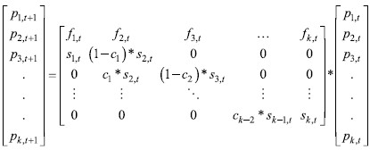 | (8) |
where ci~ Historical average ratio of last cohort age divided by population of iTH cohort.
Each ci represents the proportion of the largest age value in a given cohort. For example, if the given cohort has 100 individuals aged 10-14, where just 20 members are aged 14, then the value of ci in that cohort is 0.2. Let us say that the survival rate for the same cohort is 99% (mortality rate is 1%). This means that the next year we will see 99 individuals from this cohort. All of them are now one year older, meaning that those that were aged 14 are now aged 15 and should be put into the next cohort. In this new model, the population that is sent in next cohort is ci * si+1,t (ci does not exists for the first cohort – newborns). It starts from the second cohort, which is why we multiply its value by iTH + 1 (survival rate). The result is 0.198 (0.2*0.99), which equals 19.8 individuals. The population that stays in the same cohort equals (1 – ci) * si+1,t which in our case equals 0.792 (0.8*0.99) or 79.2 individuals. The total amounts to exactly 99 individuals (19.8+79.2). By setting the model in this way, we are setting survival rates to be uniformly distributed in each cohort, which is the assumption behind this model.
Now that we understand the changes in the model, we need to estimate parameters ci. I estimated them with the equation 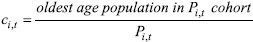
We have 17 points in time, so we estimate 17 values of ci,t for 17 different cohorts. All ci,t parameters are stationary through time, and the standard deviation value is less than 1% for almost all of them. There are just three observations of ci,t whose standard deviation is higher than 1%, around 1.5%. This is why I have decided to base the value of ci on the historical average for each cohort.
Now we can generate a stochastic forecast for the Croatian population over the next 43 years (starting from 2017). Figure 16 is the final result of 500 stochastic simulations based on the Leslie model.
Figure 16Stochastic forecast of the Croatian population from 2018 to 2060 DISPLAY Figure Figure 17Histogram of the Croatian population in 2060 forecast by using the stochastic method on the Leslie model DISPLAY Figure
The expected population in 2060 is 3.5 million and the population’s median lies around 3.49 million. The standard deviation of the total population in 2060 is 60,300, meaning 1.72% of the mean. The mean is not uncertain, as can be seen in Figure 17. Therefore, we can say with 95% confidence that the interval lies between 3.41 million and 3.65 million, and with 99% confidence that the interval lies between 3.4 million and 3.7 million. We are also interested in the changes in population for two different population groups: those aged 65+ and those aged 15-65. Figures 18 and 19 show the results of this forecast. The observable results are giving rise to growing concerns.
In the next paragraph, we are going to analyse the sustainability of the Croatian pension system through time based on the forecast population numbers. The results estimated in this paragraph will be taken in order to analyse the sustainability of the pension system.
Figure 18Stochastic forecast of the population aged 65+ from 2018 to 2060 DISPLAY Figure Figure 19Stochastic forecast of the population aged 15-65 from 2018 to 2060 DISPLAY Figure
4 Population of pensioners
Now that we have estimated the population projections for each cohort, we are able to use those estimations to analyse the population of pensioners and of the employed population. The given numbers can help us estimate how much cash inflow will be generated from the employed population and see whether there will be enough cash accumulated to finance the pensioners. This section will deal with calculating the population of pensioners in Croatia.
The pensioner dynamics behaviour can be explained through the values of already existing pensioners and new pensioners. A model can be set in the following way (Tian and Zhao, 2016):
| Pp,t = θt * Pp,t-1 + α1 * Pi,t * X1 + α2 * Pi,t * X2 | (9) |
| Pp,t = θt * Pp,t-1 + α * Pi,t * X | (10) |
Pp,t ~ Population of pensioners at time t θ ~ Survival rate of pensioners α, X ~ Scaling factor Pi,t ~ Population of iTH cohort at time t
This model calculates the number of the next year’s pensioners by adding the number of pensioners that survive this year and newly added pensioners together. As mentioned above, until 2027 women and men can retire at different ages. We therefore have two different equations necessary for catching up to the dynamics of the system. Equation (9) is used before 2027 and Equation (10) is used after 2027. At the present moment, women can start receiving pension benefits at the age of 62. In order to estimate the number of newly retired women, we first need to know what population of women is aged 62 and is eligible for a pension. We need to take into consideration the fact that not all women with these characteristics are necessarily going to retire, which is why we multiply the whole thing with X in order to get the number of women that will be new pensioners. The same procedure is used for men, and after 2027 for the total population. This model does not account for people in early retirement, so I will put them in the category with other pensioners. Now I will briefly explain and estimate the parameters, one by one.
The parameter θt represents the survival rate of pensioners. Since we already have estimated survival rates for each cohort, I estimated θt as a weighted average of survival rates in different cohorts. The survival rates of the cohorts 65+ are used because the assumption is that individuals older than 65 are pensioners. Although women may currently legally receive pension at the age of 62, θt represents the approximation of survival rates. Although after 2033 individuals will need to be 67 years old to receive pension benefits, I decided not to complicate the model further, so that θt represents the weighted average survival rates of the cohorts 65-69, 70-74, 75-79 and 80+. θt is set in the following way:
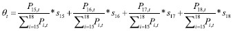 | (11) |
After the survival rates we need to analyse the scaling factor α. Term Pi,t must be multiplied by 0.5 for the years leading up to 2027 because we assume that the population consists of a 50:50 ratio of men and women. By multiplying with 0.5, we scale the population of a cohort to represent just the population of women (or men). Since only women aged 62 can start receiving pension benefits, we need to multiply the calculated value with the percentage of the population aged 62 in a given cohort in order to scale the population to just the number of women aged 62. Since we need to estimate in what way postponing the age limit for retirement affects the pension system, we need to create a method that will cover postponing the retirement age inside each cohort. There are data available for each year’s population on Eurostat, so I decided to calculate the historical average ratio of each age group for the given cohort. Table 10 shows the results for the relevant ages.
Table 10Proportion of specific age population in cohorts 60-64 and 65-69 DISPLAY Table
We can observe just what we expected – a decreasing pattern of the population for every age in the cohort. Now we have everything necessary for calculating the α parameters. When we are dealing with population of men and women separately, we multiply the numbers in Table 10 with 0.5 according to Formula (9), otherwise we keep the original numbers from Table 10 and we use Formula (10).
Up until now we calculated the number of women aged 62 (and men aged 65). Now we need to find out how many women aged 62 will start their retirement plan. Fortunately, the Croatian Pension Insurance Institute (HZMO) has been publishing the numbers of new pensioners, both female and male, since 2006. Since we have the data for women aged 62 from Eurostat, we can calculate the ratio of new female pensioners to female population aged 62 (and the ratio of new male pensioners to male population aged 65). The results for both men and women can be found in Table 11.
Table 11Analysis of new pensioners DISPLAY Table
The result of some observations is higher than one because the category new pensioners does not include only women aged 62 and men aged 65, but also people that have retired early or late. However, this ratio can be a good benchmark for forecasting the numbers of future new pensioners. I will furthermore assume that this ratio does not change with the cohort, but rather that it just changes over time. This assumption allows me to create a stochastic process of the ratio and use it for different cohorts. In Figures 20 and 21 we can see the PACF for the process created from those two ratios. I decided to use the AR (1) process to explain the future behaviour of the ratio. Table 12 shows the estimated equations.
Figure 20PACF for the ratio of new male pensioners to male population aged 65 DISPLAY Figure Figure 21PACF for new female pensioners to female population aged 62 DISPLAY Figure Table 12AR (1) process for ratio of new female/male pensioners to female/male population aged 62/65 DISPLAY Table
Now I set the two processes as yt = 0.16289 + 0.824202 * yt-1 + 0.1421 * εt and yt = 0.350618 + 0.67092 * yt-1 + 0.1437 * εt, where εt~Normal(0,1). In Figures 22 and 23 we can see the result after 500 simulations.
Figure 22Stochastic forecast of new male pensioners ratio from 2018 to 2060 DISPLAY Figure Figure 23Stochastic forecast of new female pensioners ratio from 2018 to 2060 DISPLAY Figure
The processes deviate significantly from their expected value. However, this should not pose a problem because it is our end goal to get a wider picture of the whole system. We have now estimated all the necessary parameters for forecasting the number of pensioners. Figure 24 shows the estimated results. The simulation is programmed in such a way as to incorporate the dynamics of shifting the minimum retirement age. The expected number of pensioners in 2060 is 1,211,136. We can say with 95% confidence that the interval lies between 1,073,076 and 1,349,965. These numbers will be used for further analysis. The number of pensioners at the end of 2017 was 1,236,258, which is to say that this model estimates a lower number of pensioners by 2060. The overall distribution of pensioners in 2060 can be observed in Figure 25.
Figure 24Stochastic forecast of the number of pensioners from 2018 to 2060 DISPLAY Figure Figure 25Distribution histogram for the number of pensioners in 2060 DISPLAY Figure
5 Employed population
We now need to estimate the employed population. The model of the employed population is set as follows (Tian and Zhao, 2016):| PE,t = Pw,t * lt * (1 - ut) | (12) |
PE,t ~ Employed population at time t Pw,t ~ Total working age population at time t lt ~ Labor force to working age population ratio at time t ut ~ Unemployment rate at time t
This model is very straightforward. The total working age population multiplied by the ratio of the labour force to total working age population and employment rate gives us the number of employed individuals.
The parameter lt represents labour force ratio at time t. The Croatian Bureau for Statistics has been publishing monthly data on the size of the labour force since 2003. Since data for 2018 is available, we will use it. By calculating the average of the monthly labour force numbers in a year, I can estimate the labour force for the year. By dividing the result with the working age population for the chosen year, we obtain the ratio of the labour force to working age population. I calculated the working age population as male population aged 15 to 65 and female population aged 15 to 62. Figure 26 shows the results.
Figure 26Labour force to working age population DISPLAY Figure
Since the ratio changes over time, we need to forecast its future values for the next 43 years. It is very hard to know what is going to happen in the Croatian economy over the next 5 years, let alone the next 43 years. Two other problems are that, first, the size of the working age population will fluctuate every year. Secondly, from 2033 onwards the new working age population will approximately be people aged 15 to 67. I will assume that the ratio is not dependent on the cohorts used to calculate working age population, but rather just on time. For the sake of simplicity, I will exclude the random walk hypothesis here. Figure 27 shows the PACF for the ratio of labour force to working age population. We conclude that an AR (1) process is the best fit for explaining the behaviour of the ratio 2. Table 13 shows the estimated values of the process. Afterwards I calculated the stochastic process for yt = 0.109315 + 0.827804 * yt-1 + 0.0152 * εt, where εt~ Normal(0,1), 500 simulations of which are displayed in Figure 28.
Figure 27PACF of labour force to working age population ratio DISPLAY Figure Table 13AR (1) process of labour force to working age population ratio DISPLAY Table Figure 28Stochastic forecast of labour force ratio from 2018 to 2060 DISPLAY Figure
As it is already problematic to estimate the numbers of the future labour force, it is even more problematic to estimate the future unemployment rate over the next 43 years. It is very hard to predict what the movement of the future unemployment rate in the next 43 years will be, so we need to use forward-looking techniques to estimate it. Historical unemployment rates can be seen in Figure 29. Again, we have available data for 2018, which I will use. Historically, the rates fluctuate between 10% and 20%. The year 2018 saw the lowest unemployment rate in history, estimated at 9.8%. In order to try to forecast future unemployment rates up until 2060, I will employ scenario analysis with three separate scenarios, each of which will then be used in further analysis.
Figure 29Historical unemployment rate in Croatia DISPLAY Figure
In the first scenario the average unemployment rate will dynamically return to its historical average rate. This dynamic behaviour is shown in Figure 30. Its mean expected values will be used in further analysis.
Figure 30Forecast of the future unemployment rate: Scenario 1 DISPLAY Figure
In the second scenario, I will assume that the unemployment rate will on average stay at its current levels – at 9.84%. For the third scenario, I will assume that the unemployment level will dynamically converge to 5%, by dropping by 0.5% each year. After 10 years it will stay at 5% up until 2060. Those three scenarios allow us to cover three possible movements that could occur in the Croatian economy, which will help us see the wider picture of the pension system.
After creating a program that dynamically includes the postponement of the retirement age and simulating results according to Scenario 1, the results for the employed population over time can be seen in Figure 31. The expected size of the employed population in 2060 is 1,082,232. The employed population is thus smaller than the population of pensioners. This indicates the possibility that there will be high pressure on government expenses for the pension system in 2060.
Figure 31Stochastic forecast of the employed population: Scenario 1 DISPLAY Figure
Figure 32 shows the dynamics of the employed population generated according to Scenario 2. The expected employed population in 2060 is 1,153,739, which is 71,500 people more than in the last scenario. Furthermore, this number is still lower than the expected number of pensioners.
Figure 33 shows the expected employed population over time according to Scenario 3. The expected employed population in 2060 is 1,215,739, which is higher than the expected pensioner population in 2060. Since the expected number of pensioners in 2060 is 1,211,136, the best possible scenario is to end up with a 1:1 ratio of worker to pensioner by 2060.
Figure 32Stochastic forecast of the employed population: Scenario 2 DISPLAY Figure Figure 33Stochastic forecast of the employed population: Scenario 3 DISPLAY Figure
6 Analysis of sustainability
Before answering the question of sustainability, we need to set the benchmark for what a sustainable system is. Let us first consider how the system functions. A certain number of people work and earn a salary for their work. A percentage of that gross salary is paid towards the pension system. This money is then used in two ways – it provides current pensioners with a pension and it is invested for capital accumulation. Therefore, a certain percentage of this money goes directly to the government for already existing pensioners. The government is obliged to provide retired individuals with pensions. So, our question is: can the government generate enough cash flow from the employed population in order pay out pensions? If the cost of paying the pensioners is higher than the revenue earned, the government needs to pay for the rest with its own money or borrow money, so this could be understood as an investment. As opposed to companies, when the debt or cash outflow of a government is increased, every citizen is affected one way or another. Therefore, it is of the utmost importance to analyse the investment in the pension system. If the overall expenses are not too high, it will remain in the government’s interest to pay for the pension system since it positively affects social conditions. However, only up to a certain point. Just as with companies, there are levels of debt where the government is better off not investing. In order to find out at what cost level the government is at break-even point requires a rather complex analysis, since many factors play vital roles. In 2017, the Croatian government gained 21.09 billion Kuna (HRK) revenue from the pension system and incurred HRK 37.67 billion expenses for the pension system (Mirovinsko.hr, 2018). The net amount was HRK -16.58 billion, whereupon the new reform was started. For this reason, I will use HRK 16.58 billion as the benchmark where the government is better off not investing. If the present value of future net expenses is higher than HRK 16.58 billion, it will be interpreted as unsustainable. It must be mentioned that this interpretation of unsustainability comes along with the assumption that the economic conditions in the country are not going to change in the next 43 years. This is not to be expected, but since I cannot know whether the economy will expand or weaken unexpectedly in the future, I decided to use this number for further analysis. I will compare the calculated present value of future expenses with 16.58 billion.
In order to forecast future government revenues and expenses from the pension system, we need to forecast wages in the country (Tian and Zhao, 2016). Table 14 shows the average gross salary and growth rates for each year. In later analysis, I shall exclude the values from 2018, but they are displayed in this table.
Table 14Average gross salary and growth rates DISPLAY Table Figure 34PACF of growth rates in wages DISPLAY Figure
The average growth rate of the gross salary is 3.1%. From Figure 34 we conclude that the autocorrelation function of the first order should be used in order to predict future growth rate values. By knowing the future growth rate values, we can easily calculate future salary values. It is hard to predict future salary growth rates over the next 43 years. Growth rates can be explained through the economy of the country, as well as through politics and law. Most of those variables are hardly observable in the economy. I will use the AR (1) model to estimate the parameters. Since we are forecasting 43 years ahead, as long as we use the correct average and take various possible events and extrema into consideration, we should get a very good dynamical convergence of the salaries. Table 15 shows AR (1) parameters estimates. Now I created the following process: yt = 0.0143 + 0.52176 * yt-1 + 0.0264 * εt, where εt ~ Normal(0,1). Figure 35 shows the result of 500 simulations of the process.
Table 15AR (1) process for growth rates in wages DISPLAY Table Figure 35Stochastic forecast for growth rates in wages DISPLAY Figure
The process estimates growth rates between -10% and 15%. I believe that the 500 simulations generated above can explain the dynamics of future growth rates in wages for the next 43 years. Figure 36 shows the realized values of future wages. The expected gross wage in 2060 is HRK 29,735 and the median value is HRK 28,343. Estimated wage distribution in 2060 can be seen in Figure 37. We can estimate with 95% confidence that the interval lies between HRK 15,106 and HRK 51.307.
Figure 36Stochastic forecast of future wages DISPLAY Figure
Now we can start estimating the revenues generated from the pension system over the next 43 years. We know that before 2019, 15% (contribution rate) of an individual’s gross salary was paid to the first pillar 3. That money was then used to finance pensioners. After the new reform, every pensioner may decide whether they want to receive a combined pension (financed from both pillars) or a firstpillar pension only. We can conclude that the combined pension scheme was not sustainable, since the government implemented its reform in 2019. If an individual wants to receive pension just from the first pillar, all the capital accumulated in the second pillar will be transferred to the state.
Figure 37Histogram of wage distribution in 2060 DISPLAY Figure
Now we need to estimate the amount of capital accumulated in the second pillar and that may be a difficult problem. Firstly, recall from the first paragraph that individuals can decide which investment scheme they want to have in the second pillar. Each investment scheme leads to different capital accumulated. Forecasting the future expected returns and standard deviations is a problem that requires deeper stochastic analysis which I will not implement here. Secondly, each year, a different number of individuals will decide to send their capital from the second pillar to the state, and we can view the number of individuals in each year as a random variable through time i.e. stochastic process which I will not model here. Putting everything together, future expected returns of the second pillar and the number of individuals that decide to receive pensions just from first pillar can be modelled as a stochastic process, but I will not involve stochastic calculus here; it is left for future research.
We do know that the market-implied pension contribution rate lies between 15% and 20% from the fact that some individuals will receive a combined pension and others will receive pension just from the first pillar. Therefore, I will estimate future revenues by setting my equation in such a way that the contribution rate equals to 20%, meaning that 20% of the gross salary is paid towards the government after January 1, 2019. If every individual decided to receive their pension just from the first pillar, estimating the contribution rate at 20% is a very good approximation of government cash flow through time. The equation for calculating revenues is set in the following way (the revenues are scaled to a yearly basis) (Tian and Zhao, 2016):
| Revenuest = Average gross waget * Employed populationt * 0.2 * 12 | (13) |
When it comes to expenses, we need to know what percentage of the gross wage the pension should amount to. Table 16 shows the average pension rates for December of each year, as reported by HZMO, as well as the percentage of the average gross salary in that year.
Table 16Average pension by year and percentage in gross salary DISPLAY Table
As we can see, the percentage of the pension amount in gross salary oscillates between 28% and 33%. The average is 30%, so I will use that value as the expected pension per pensioner in further analysis. This wage indexation is assumed for reasons of simplicity in further analysis. The expenses equation is set in the following way (Tian and Zhao, 2016):
| Expensest = Average gross waget * Pensionerst * 0.3 * 12 | (14) |
This equation is also scaled to yearly values. By subtracting costs from revenues, we obtain the net cash flow generated from the pension system. We again have three different scenarios, which will be analysed separately.
If we use the contribution rate of 15% in Equation (13), we estimate that the expected net cash flow in 2018 is HRK -16.1 billion. We already know that in 2017 the net cash flow was HRK -16.58 billion. As already mentioned, since the start of 2019, every individual has been able to decide whether they want to their pension to be funded from the first pillar or be combined, which will directly influence the contribution rate. If we assume that no one will use the combined pension system, we can exclude its existence from our calculations – to simplify the estimation process – and say that 20% of the salary amount will be contributed just for the first pillar.
In all three following scenarios, analysed in paragraphs 6.1, 6.2 and 6.3, I expect that the second pillar will not gain enough competitiveness in comparison with the first pillar. This is just an assumption in order to see what the outcome of this scenario is, and readers should be aware of it. Later, the outcome of the scenario when the second pillar gains in competitiveness will be shown.
6.1 Future dynamics of the pension system without the second pillar: unemployment rate Scenario 1
As described above, in the first scenario the unemployment rate is expected to return dynamically to its historical average. We have already concluded that this is the worst-case scenario when it comes to the ratio of pensioners to workers. We can thus expect that this scenario will also be the worst in net cash flow generated by the government from the pension system. The result calculated by estimating revenues and subtracting estimated expenses can be seen in Figure 38. The expected net cash flow in 2060 is HRK -53.91 billion. Discounted until today with discount factor of 2.99%4 – since the expected wage growth is 2.99% per year (as shown in Table 15) – we obtain the value of HRK -15.19 billion. This number is very close to the value of HRK -16.58 billion, meaning that it is showing signs of possible unsustainability. The future value of HRK 16.58 billion in 2060 is HRK 58.9 billion (calculated with an interest rate factor of 2.99%). The percentage that corresponds to the value of HRK -58.9 billion is around 34%. We can interpret this by saying it is 34% probable that the pension system will be unsustainable by 2060 if the unemployment rate converges to its historical average.
Figure 38Stochastic forecast of government net cash flow from the pension system: Scenario 1 DISPLAY Figure
6.2 Future dynamics of the pension system without the second pillar: unemployment rate Scenario 2
In the second scenario, the unemployment rate is expected to oscillate around 9.84%, which equals to the value of the average unemployment rate in 2018. We already know that in this case the net cash flow generated from the pension system should be positively affected. Figure 39 shows the net cash flow generated from the pension system. The expected net cash flow in 2060 is HRK -48.81 billion. The present value of HRK -48.81 billion is HRK -13.75 billion. The percentage that corresponds to the value of HRK -58.9 billion is around 23%. So we can say that it is 23% probable that the pension system will be unsustainable by 2060 if the future unemployment rate oscillates around 9.84% on average. Considering that the historical unemployment rate was never this low, if it stayed at this level for the next 43 years, 23% of the simulated results (out of 500) leads to government debt that we consider unsustainable. This is not a good outlook for the Croatian pension system. The truth is that the historical unemployment rate has nothing to do with the future unemployment rate, so it is feasible to assume that the unemployment rate could actually be at this level, if not at an even lower one.
Figure 39Stochastic forecast of government net cash flow from the pension system: Scenario 2 DISPLAY Figure
6.3 Future dynamics of the pension system without the second pillar: unemployment rate Scenario 3
In the third scenario, the future unemployment rate is expected to oscillate around 5% on average. We already know that this is the best scenario out of the three that are created. Figure 40 shows net cash flow generated by the government if scenario 3 occurs. The expected net cash flow generated in 2060 is HRK -44.38 billion which equals HRK -12.50 billion at present value. The percentage that corresponds to the value of HRK -58.9 billion is around 17%. Figure 40 shows that the expected net cash flow may not change that much over the next 15 to 20 years. But after 2040 the expected net cash flow starts to decrease rapidly.
Figure 40Stochastic forecast of government net cash flow from the pension system: Scenario 3 DISPLAY Figure
We are interested in the present value of future expenses. An interesting phenomenon can be observed from Figure 41. The figure shows the expected present value of future expenses over the years. With the unemployment rate from Scenario 3, we can notice that the present value of future cash flow keeps increasing over the first 12 to 15 years. It then starts decreasing without signs of stopping. This expected present value of future cash flow is estimated if the contribution rate equals to 20%, meaning that every individual decides to receive pensions just from the first pillar. Figure 41 predicts that this reform will not solve financial sustainability problems; it will only postpone them for a couple of decades.
Figure 41Expected present value of government future cash flow generated from the pension system: Scenario 3 DISPLAY Figure
These three analysed scenarios were created on the assumption that the second pillar of the pension system will never be as competitive as the first pillar. Next, we will analyse what would happen if the second pillar gains in competitiveness. It should be mentioned again that this interpretation of unsustainability is made with the assumption that the economy will not change a lot from its present state. If a huge positive shift in the real gross domestic product (GDP) happened, then the government could handle higher debt for the pension system. This interpretation of unsustainability should be understood by its being kept in mind that I can hardly predict future changes in the economy.
6.4 Strengthening the second pillar
In this chapter there will be an assumption of the fungibility of the first and second pillar in order to estimate the fiscal space that could be opened to raise the replacement rates. The second assumption is that the second pillar will not be immediately strengthened in 2019. I will assume that the strengthening of the second pillar will occur in 2030. This assumption may be questionable but thinking of the dynamics of the system we can conclude that the new reform will not immediately affect the financial sustainability of the pension system in 2019, but rather it will take some time until the dynamics adjust. Therefore, I created scenarios in which the second pillar is staring to gain strength in 2030. If the assumption is made that second pillar is starting to gain strength in 2025 or 2035 the overall solution deviates less than 1% from what will be illustrated in this paper, which indicates that as long as the second pillar gains strength in the forecast period the convergence in the solution is inevitable. Therefore, in 2030 pensioners will decide to receive their pension from a combined pension scheme and the new contribution rate will be 15%. For this case I will create two different scenarios. In the first scenario, the government will pay 75% of the total pension amount, since the contribution rate of 15% equals 75% of the total pension amount. The other 25% will be financed from the second pillar. In the second scenario I expect even better strengthening of the second pillar, where the same conditions regarding this year apply as in the first scenario, but I will also assume that every two years the government will decrease expenses by 5% over the next ten years. Government expenses for the total pension system would remained fixed at 50% after 2040. The other 50% will be financed from the second pillar (note that the assumption of the fungibility of the first and second pillar is used).
For the first scenario, revenues and expenses are set in the following way:
| Revenuest = Average gross waget * Employed populationt * 0.15 * 12 | (15) |
| Expensest = Average gross waget * Pensionerst * 0.3 * 12 * 0.75 | (16) |
These equations are applied for the years after 2030.
In this scenario, the government is earning less revenue, but it is also incurring fewer expenses. Figure 42 shows the estimated result of a stochastic forecast of the government net cash flow, where the unemployment rate is expected to increase over the years (scenario 1 for the unemployment rate). In 2060, the expected net cash flow is HRK -40.43 billion, which stands for HRK 11.39 billion present value. This is already a better result than the one analysed in paragraph 6.3. The percentage that corresponds to the amount of HRK -58.9 billion 2060 is around 12%.
Figure 43 shows the estimated result of net government cash flow generated with Equations (15) and (16), where the unemployment rate is expected to decrease over the next 43 years and remain around 5%. The expected net cash flow in 2060 is HRK -33.28 billion, which stands for HRK -9.38 billion present value. The percentage that corresponds to the value of HRK -58.9 billion in 2060 is around 5%. We can conclude that if the second pillar gains in competitiveness, we can expect stronger financial sustainability of the Croatian pension system.
This analysis shows that possible strengthening of the second pillar would exert much more influence on the whole pension system than changes in the unemployment rate. According to this scenario, we can say that there it is 5% to 12% probable that the Croatian pension system is unsustainable by 2060 if the second pillar shows enough strength to cover 25% of the total expenses created by the pension system. This interpretation of unsustainability comes along with the assumptions we set in this analysis.
Figure 42Stochastic forecast of government net cash flow with the assumption that pensioners decide to use a combined pension scheme after 2030. Unemployment rate from scenario 1 is used DISPLAY Figure Figure 43Stochastic forecast of government net cash flow with the assumption that pensioners decide to use a combined pension scheme after 2030. Unemployment rate from scenario 3 is used DISPLAY Figure
For the second scenario of strengthening in the second pillar, the used expenses equation changes dynamically through time, starting as Equation (16). Every 2 years the expenses drop by 5%, so that the equation for the years after 2040 is set in the following way:
| Expensest = Average gross waget * Pensionerst * 0.3 * 12 * 0.5 | (17) |
Figure 44 shows the estimated net government cash flow generated by this scenario. This figure shows financial sustainability of 100%. The expected government net cash flow in 2060 is HRK -7.64 billion. This is so far the best possible scenario that can occur. Also, around the year 2040, the expected government net cash flow for the pension system has positive values. If the second pillar gained enough strength to replicate this scenario, there would not be a single observation that yields financial unsustainability. Figure 44Stochastic forecast of government net cash flow with the assumption that the second pillar gains enough competitiveness to cover 50% of expenses after 2040. Scenario 1 unemployment rate is used DISPLAY Figure
6.4.1 Can pension increase if second pillar gain its competitiveness?
We saw that if we expect the unemployment rate to increase on average in the forecast horizon, and if the second pillar gains enough competitiveness to cover 50% of the expenses of the pension system, then the pension system would surely be financially stable in the forecast horizon. If the average unemployment rate stays at the same value as in 2018 (9.84%) or if it decreases in the forecast horizon, the result will be even better. In this scenario we expected pensions to amount to 30% of the gross salary. We saw that the pension system is definitely sustainable in this scenario, no matter what the unemployment rate is.
Together with assumption of the fungibility of the first and second pillar, I assume that pensions will amount to 35% of the gross salary after 2030 with the unemployment rate from scenario 1 (where the unemployment rate increases over time), and financial sustainability is 100% probable. The worst observation generated by this scenario is HRK -51.28 billion in 2060, which is still lower than the future values of HRK -16.58 billion. We can conclude that if the second pillar generates enough competitiveness to cover 50% of the expenses after 2040, then the government will be able to increase the pensions to 35% of the gross salary, and the system will still be financially sustainable with 100% probability.
Figure 45 shows the stochastic forecast for net cash outflow if we add another extra condition to the previous scenario: that pensions amount to 40% of the gross salary after 2040. The expected government net cash flow in 2060 is then HRK -28.55 billion. The percentile that corresponds to the value of HRK -58.9 billion is around 1%. This was calculated with the worst unemployment rate scenario. According to this analysis, the government would be able to increase pensions to amount to 35% of the gross salary between 2030 and 2040. They would also be able to increase them once more in 2040 to amount to 40% of the gross salary with a maximum of 1% probability of being financially unsustainable. If the second unemployment rate scenario occurred, the expected probability for the system to be unsustainable is less than 1%. If the third unemployment rate scenario occurred, the expected probability for the system to be unsustainable would be around 0.1%. The results of this analysis are based on the assumption that the second pillar gains enough competitiveness to cover 50% of the expenses of the pension system.
Figure 45Stochastic forecast of government net cash flow with the assumption that the second pillar gain enough competitiveness to cover 50% of expenses and extra assumption that pension amounts to 35% of gross salary between 2030 and 2040 and 40% of gross salary after 2040. Scenario 1 of unemployment rate is used DISPLAY Figure
7 Conclusion
In this paper I used stochastic methods to analyse the sustainability of the Croatian pension system. I also created three possible scenarios for future unemployment rates: A scenario in which the unemployment rate will on average increase for the next 43 years, a scenario where the unemployment rate will on average stay the same as it was in 2018, and a scenario where the unemployment rate will on average decrease.
The benchmark of unsustainability is the net cash flow in 2017, HRK -16.58 billion, since it was after that year that the government started working on the new reform. If the present value of future net cash flow is lower than HRK -16.58 billion, the pension system is said to be unsustainable. This is made with the assumption that Croatia will not experience significant unexpected positive or negative shifts in the economy in the forecast period.
Furthermore, I created three scenarios to forecast future movements in the pension system. In the first scenario, the second pillar never gains enough competitiveness to compensate pensions generated from the first pillar, meaning that every individual would receive pensions just from the first pillar. The analysis demonstrated that there is a between 17% and 34% chance that the pension system will be unsustainable by 2060 if this scenario occurs.
In the second scenario, the second pillar gains enough competitiveness after 2030 to compensate for the same value of pensions as the first pillar. So that the expected cost of pension system is financed 75% by the first pillar and 25% by the second pillar. This scenario demonstrated that there is 5% to 12% probability of the pension system being financially unsustainable.
The third scenario is set in such a way that the cost of the pension system in 2030 is financed 75% by the first pillar and 25% by the second pillar. After 2030, I assumed the fungibility of the first and second pillar in such a way that more than 25% of the individual pension is financed from the second pillar. This indirectly estimates the fiscal space that could be opened to raise the replacement rates. The amount paid for the pension system by the first pillar is reduced by 5% every two years until 2040. In 2040, the costs of the pension system are split evenly between the first and second pillar. It was demonstrated that in this scenario there is a 100% probability that the pension system will be financially sustainable by 2060.
It was also demonstrated that if the second pillar gained enough competitiveness to cover 50% of the expenses after 2040, the expected pension rates (replacement rate) could be increased to 35% of the gross salary after 2030 with 100% probability of being financially sustainable. Furthermore, it was shown that an extra increase in the pension rate – where it would amount to 40% of the gross salary after the year 2040 – is possible in this scenario, with a 1% probability of being financially unsustainable, all while taking into account the worst unemployment rate scenario.
Notes
* The author would like to thank two anonymous referees for their valuable comments and suggestions.
1 This paper concludes that fertility rates would improve based on AR(1) process. AR(1) is not greatest approach one can use in estimating fertility rates because there are too many other factors which AR(1) process does not pick and future work could improve its forecasting.
2 Using AR(1) process to project labor force to working age population ratio inertially projects past trends to future activity levels and probably undershoots the future (elderly) employment levels and contribution revenues that would result from pension policy and longer activity. The reader should be advised of this and possible upgrades of the model in the future.
3 Author’s note: This is not true for everyone, but we want to simplify the calculation process.
4 Discounting with wages was used instead of GDP for reasons of simplicity i.e. GDP is assumed to grow at the same rate.
Disclosure statement
No potential conflict of interest was reported by the author.
References
Cull, P., Flahive, M. and Robson, R., 2005. Difference Equations: From Rabbits to Chaos. New York: Springer.
Enders, W., 2014. Applied Econometrics Time Series. New Jersey: Wiley.
Puljiz, V., 2007. Hrvatski mirovinski sustav: korijeni, evolucija i perspektive. Revija za socijalnu politiku, 14(2), pp. 163-192 [ CrossRef]
Smith, S. K., Tayman, J. and Swanson D. A., 2013. A Practitioner’s Guide to State and Local Population Projections. New York: Springer.
Tian, Y. and Zhao X., 2016. Stochastic Forecast of the Financial Sustainability of Basic Pension in China. Sustainability, 8(46), pp. 1-17 [ CrossRef]
|


