|
|
|
Abstract
In this paper, we study whether taking into account non-income dimensions along with income while measuring individual well-being matters for cross-country welfare comparisons. We focus on the 27 EU member states over the period 2007-2011, using data from the European Quality of Life Survey. Individual well-being is measured by equivalent income, which is equal to the actual income minus the monetary value of suffering from not having the best achievements in non-income dimensions. Cross-country comparisons of these statistics and their growth rates show that going “beyond income” makes a substantial difference. In particular, we find that when social welfare is measured by an index sensitive to both mean well-being and its inequality, leaving out non-income dimensions, especially health, from well-being measurement, would leave unexplained more than half of the cross-country variation in social welfare. Taking non-income dimensions into account affects more the part of social welfare that is inequality-sensitive than the one that is mean sensitive.
Keywords: well-being; multi-dimensional; equivalent income; social welfare; non-income dimensions
JEL: I30, D31, D63
1 Introduction
Improving social welfare – providing better lives for citizens – is a proclaimed, if not always achieved, objective of any society. Mainly due to practical purposes, social welfare has been for long dominantly identified with some measure of aggregate national output or income. Gross domestic product (GDP) per capita is still predominantly used as a measure of countries’ overall welfare. This comes from the commitment to the idea that income creates real opportunities for a good life. The importance of non-income dimensions, is acknowledged only indirectly. Another feature of the dominant approach in measuring social welfare is that the distribution of social welfare has been relatively neglected, at least until recently. This is best reflected in the high importance attached to the efficiency aspect of social welfare relative to its equity aspect.
The recognition of excessive focus on income has been around at least since Sen (  1985 1985). He conceptualised well-being of a person as the extent of her “capabilities”, meaning her real freedom to achieve “functionings” that she reasonably values. Effectively, this amounted to recognising multi-dimensionality of individual wellbeing and the need to measure it directly, rather than assuming that higher income will generate a larger set of functionings. Based on these ideas, the United Nation Development Programme (UNDP) created a Human Development Index (HDI) that consists of three dimensions: GDP per capita, literacy and longevity. Recently, the recognition that well-being is multi-dimensional and should be measured accordingly has gained momentum, largely due to the influential Stiglitz-Sen-Fitoussi Report (Stiglitz, Sen and Fitoussi, 2009). They criticise the “GDP approach” and accordingly they recommend going beyond it (Stiglitz, Sen and Fitoussi, 2010). The Organization for Economic Cooperation and Development (OECD) also recognizes the multi-dimensional notion of well-being. Operationalising one of the organisation’s “key priorities”, namely to measure quality of life and monitor broader notions of social progress, in 2011 the OECD launched the “Better Life Initiative” (OECD, 2011). The importance of accepting multi-dimensional well-being has been recognized as well by the European Commission, which in 2009 issued the communication “GDP and Beyond”, and took steps to collect data for the construction of a multi-dimensional measure (ESS, 2011). This issue has thus reached the European political agenda (Bache, 2013).
In this paper, we go beyond income in assessing well-being in 27 European Union (EU) member states 1 over 2007-2011. 2 We ask whether the way in which wellbeing is measured makes any difference for cross-country well-being comparisons. To do so, we start from the individual, rather than the societal level. We use individual data from a wide European survey to construct, for each individual in a given country and year, a multi-dimensional well-being measure combining income with five non-income dimensions: health, unemployment, housing quality, crime and environmental quality. We also go beyond the mean, by assessing well-being inequality along with its mean level.
The multi-dimensional well-being measure that we use is equivalent income. It is defined and discussed in a number of papers, but here we refer to the most recent and detailed papers of Decancq, Fleurbaeyn and Schokkaert ( 2015a; 2015b) and Fleurbaey ( 2015). For a person with some income and non-income dimensions, equivalent income is the hypothetical amount of income which, when combined with the best (most preferred) levels of all non-income dimensions, gives this person the same utility as her actual income and her actual achieved levels of nonincome dimensions. The relative weights assigned to income and non-income dimensions are not arbitrary (e.g., equal weights) but rather derived from preferences of the population. We estimate preferences using a model of life satisfaction. Precisely, a life satisfaction score is regressed on income and non-income dimensions, controlling for other correlates of life satisfaction. In doing so, we estimate the preferences held by what we could term a “representative EU citizen”, where “representative” refers to the fact that preferences are homogeneous and estimated on a sample representative of the EU population.
Although subjective well-being scores are used to construct it, equivalent income is a non-welfarist measure with cardinal properties and it is directly comparable to income. Thus, the whole toolkit of distributional analysis can be applied to income and equivalent income alike, enabling comparisons of various indicators based on incomes with those based on equivalent incomes.
Equivalent income has been used in a number of papers so far, both for single- and multi-country analyses. In an analysis based on Russian longitudinal survey data, Decancq, Fleurbaeyn and Schokkaert ( 2015a) compared equivalent income to a uni-dimensional monetary measure (expenditures per capita), life satisfaction and an objective multi-dimensional measure. They found that the identification of the worst off depends on the well-being measure used. Decancq and Neumann ( 2016) and Decancq, Schokkaert and Zuluaga ( 2016) reached similar conclusions with German and Columbian data, respectively. Decancq, Fleurbaeyn and Schokkaert ( 2017) examined different sources of equivalent income inequality in Russia and found that a large part can be explained by preference heterogeneity. Using data on Flemish adults, Defloor, Verhofstadt and Van Ootegem ( 2017) explored the robustness of equivalent income to the type of subjective well-being data used for preference estimation, and concluded that while the overall ranking of individuals is quite robust, there are certain differences in the profiles of the worst off. Jara and Schokkaert ( 2016) exploited Swedish EU-SILC data and the microsimulation model EUROMOD to show that ex-ante policy evaluations may benefit from using equivalent income as a richer well-being measure compared to disposable income. A couple of papers focused on health-related applications. Fleurbaey et al. ( 2012) and Schokkaert et al. ( 2013), using data from a French survey, proposed using equivalent income as an approach to assess socio-economic (incomerelated) equity in health, showing that it is feasible and that it may be normatively more appealing than the traditional approach based on a concentration index of health (or health care) with respect to income. In another application to health, Samson et al. ( 2017) showed that it is feasible to use equivalent income in a distribution-sensitive cost-benefit analysis, as an alternative to the traditional costeffectiveness analyses in health technology assessments.
There are also multi-country studies. Fleurbaey and Gaulier ( 2009) estimated average equivalent incomes for 24 OECD countries based on macro data and found that the ranking of countries by this measure is considerably different from the ranking by GDP per capita. With micro data for 13 countries and macro data for 152 countries, Jones and Klenow ( 2017) conclude that although the average equivalent income is highly correlated with GDP per capita, there are substantial deviations between the two. The dispersion of well-being among the developed countries is smaller than according to GDP per capita, while the less developed countries lag behind the most developed countries more than GDP per capita comparisons suggest. Decancq and Schokkaert ( 2016) used micro data for 18 European countries in 2008 and 2010 to show that conclusions about changes in overall well-being depend largely on whether individual well-being is measured by income or equivalent income and whether the social welfare function accounts for inequality.
In our analysis, we examine the average income and equivalent income, inequality of their distributions, and income- and equivalent income-based social welfare, represented by a distribution-sensitive social welfare function. We look at not only the levels of these indicators in 2007 and 2011, but also their changes between the two years. Throughout, we make comparisons between the income-based and equivalent income-based indicators in order to answer the question of whether measuring individual well-being by equivalent income, rather than by income, makes any substantial difference. In particular, we compare the magnitudes of income- and equivalent income-based indicators, the magnitudes and signs of their growth rates, and country rankings. The analysis includes a couple of decompositions. First, we decompose equivalent income inequality into the respective contributions of inequalities in income and non-income dimensions, in order to see how the well-being dimensions compare in terms of their contributions to equivalent income inequality. In particular, we are interested in how the contribution of income compares to the contributions of non-income dimensions, and how the contributions of non-income dimensions compare among themselves. Further, for both income and equivalent income, we decompose the cross-country variation in social welfare into the contributions of variation in means and variation in inequality, in order to see whether the relative magnitudes of the two sources of variation change upon switching from income to equivalent income. Finally, we decompose the cross-country variation in equivalent income-based social welfare into the contributions of variation in income-based social welfare and variation in the average achievements in non-income dimensions. This decomposition enables us to see how important including non-income dimensions is in accounting for countries’ overall well-being when it is conceptualised as multi-dimensional and distribution-sensitive.
We make the following contributions to the literature. First, this is the first paper using equivalent income where equivalent income inequality is decomposed in a straightforward way, into the contributions of income and non-income dimensions, and for multiple countries. The closest to our approach are Ledić and Rubil ( 2019) who decomposed the difference in income and equivalent income inequality into i) the vertical effect which arises from the correlation between income and non-income dimensions and between income and preferences and ii) the re-ranking effect which occurs upon changing positions between income and equivalent income distributions. Decancq and Schokkaert ( 2016) estimated equivalent income inequality for 18 countries and compared it to income inequality, but did not provide any decomposition. Decancq, Fleurbaey and Schokkaert ( 2017) decomposed inequality in equivalent income in a number of contributions, including the correlations between dimensions, inequality in particular dimensions and preference heterogeneity. However, they did that for only one country (Russia), whereas we provide evidence for a larger set of 27 countries. Second, unlike others, we quantify the contributions of cross-country variations in mean equivalent income and equivalent income inequality to the cross-country variation in equivalent income-based social welfare. In addition, we compare the results with those obtained from the same decomposition of income-based social welfare to see if the introduction of non-income dimensions changes the relative importance of the distributional (or equity) aspect of social welfare. Third, to our knowledge, we are the first to exploit the fact that, given the social welfare function we are using, the natural logarithm of equivalent income-based social welfare is a linear function of the natural logarithm of income-based social welfare and the average levels of non-income dimensions. This simple functional relationship enables us to assess the contributions of income-based social welfare and average levels of nonincome dimensions to equivalent income-based social welfare.
The results can be summarised as follows. The difference between the average income and the average equivalent income is substantial in the sense that for all countries, the latter amounts to less than half of the former. Although the ranking of countries in a given year by the mean equivalent income is very much the same as that by the mean income, the rankings by growth rates, which for most countries differ not only in magnitude (when they are of the same sign), but also by the sign, are quite different. Equivalent income inequality is much higher than income inequality, and country rankings by both the level and change in equivalent income inequality are substantially different from the respective rankings by income inequality. Non-income dimensions contribute more than income to equivalent income inequality, and among them health is by far the most important non-income dimension. Concerning distribution-sensitive social welfare, the cross-country variation in income-based social welfare is almost entirely accounted for by variation in the mean income, which is considerably less the case for equivalent income-based social welfare. The cross-country variation in equivalent income-based social welfare is dominantly accounted for by variation in non-income dimensions, health in particular. Thus, focussing only on income while leaving non-income dimensions (i.e. especially health) out of cross-country well-being comparisons amounts to neglecting a great deal and leads to a largely incomplete picture of well-being.
The rest of the paper is organised as follows. In section 2, we define equivalent income, we explain how to estimate preferences and calculate equivalent incomes. Section 3 describes the data. In section 4, we estimate the life satisfaction model and discuss the estimates. Section 5 presents the results. Summary and conclusions are in the last section.
2 Equivalent income
We need a multidimensional measure satisfying several requirements. First, the measure should be defined at the individual level so that it is possible to assign the value of multidimensional well-being to each person. This is essential for the measure to capture correlations between income and non-income dimensions or, in other words, to take into account their joint distribution. Second, it should summarise income and non-income dimensions for each person in a number, and the relative weights of the dimensions should not be arbitrary but rather theoretically justified and estimated from data. Third, it should be a cardinal ratio-scale variable so that both ratios and differences of two persons’ levels of multidimensional well-being should make sense. Fourth, it should be expressed in monetary units. All the requirements, except the part of the second one concerning weighting, are needed for the measure to be directly comparable to income at the individual level so that the standard tools of distributional analysis can be applied to both income and the measure of multidimensional well-being.
A multi-dimensional measure that satisfies these requirements is the so-called equivalent income (see Decancq, Fleurbaey and Schokkaert, 2015a; 2015b; Fleurbaey 2015). Let individual i’s well-being be a function of her income, Yi, and D non-income dimensions collected in vector Xi=(X 1i, X 2i, ... X Di) . Suppose all the non-income dimensions have well-defined best (most preferred) levels denoted by X*=( X*1, X*2, ... X*D). Let every individual have a utility function, Ui, with income and non-income dimensions as arguments, determining her cardinal utility level. With this notation, i’s equivalent income, Yi*, can be defined as | Ui(Yi, Xi)=Ui(Yi*, X*) | (1) |
The equivalent income of individual i represents her hypothetical amount of income which, when she has all non-income dimensions at the best levels, gives her the same utility level as the combination of her actual income and non-income dimensions. By the definition, if i is at the best levels of non-income dimensions, her equivalent income equals her income. The difference between i’s income and equivalent income can thus be understood as i’s willingness-to-pay ( WTPi) to have the best levels of non-income dimensions: Yi*= Yi− WTPi . Thus, for individuals i and j, even if Yi is higher than Yj, Yi* will be lower than Yj* if WTPi is sufficiently larger than WTPj.
It may seem reasonable not to bother constructing individuals’ equivalent incomes when one can just compare their utility levels. Yet doing so one would assume that individuals i and j have the same cardinalisations of their utility functions which is quite restrictive assumption to make. However, one reason why individuals can have different cardinalisations of the utility function is due to their different aspirations. A person forms aspirations relative to either herself in the past, or in the future, or her peer (or reference) group. For example, suppose two persons have the same income and health, but one of them is from a disadvantaged family where the parents were ill and thus able to earn income sufficient only for poor living standard, while the other is from a family where the parents were healthy and able to earn a high income. If the income and health of the person from the disadvantaged family are now higher than what her family enjoyed while she was growing up, she may be very happy or satisfied with her life. Indeed, even more so than the person from the well-off family who may not see her current situation as something with which she should be particularly satisfied.
The previous argument goes against using the answers to subjective well-being (happiness, life satisfaction) questions in surveys as interpersonally comparable well-being measures. However, this does not mean that the answers to such survey questions are worthless for empirical welfare analysis. As shown by Decancq, Fleurbaey and Schokkaert ( 2015a; 2015b), one can use happiness and life satisfaction data to estimate ordinal preferences, a crucial piece of information required for the construction of individual equivalent incomes. The key assumption is that the answers to subjective well-being questions contain information on ordinal preferences, although these answers may not be appropriate as a metric of individual well-being. Denoting person i’s reported subjective well-being (as a proxy for utility Ui) by Si, this premise is embodied in the “consistency assumption” (Decancq, Fleurbaey and Schokkaert, 2015a; 2015b) which says that the individual i weakly prefers, according to her ordinal preferences, combination ( Yi, Xi) over combination ( Yi', Xi') if and only if Si( Yi , Xi) ≥ Si( Yi' , X 'i). The following assumption can also be stated in a setting where two individuals with common preferences and aspirations are compared, which implies that the individuals i and j, weakly prefer ( Yi , Xi) over ( Yj, Xj) if and only if Si( Yi , Xi) ≥ Si( Yj, Xj). Essentially, since i and j have common ordinal preferences and, in addition, they have the same aspirations, they can be treated as the same person, and therefore an i nterpersonal comparison turns into an intrapersonal comparison.
For the consistency assumption to be satisfied, the subjective well-being question must be such that it asks respondents to perform an evaluation of their lives, rather than to express their affections. As argued by Decancq, Fleurbaey and Schokkaert ( 2015a; 2015b), questions asking about life satisfaction as a more evaluative concept appear in that sense better than those asking about happiness as a more affective concept, capturing also daily moods. 3 In addition, there should be a sufficiently rich set of personal characteristics related to aspirations, because leaving them out would amount to comparing subjective well-being among people with different aspirations and thus different cardinalisations of the utility function.
Provided that the consistency assumption holds and having the individual data on subjective well-being, income, non-income dimensions and characteristics related to aspirations, one can estimate ordinal preferences by estimating the parameters of an econometric model in which subjective well-being is modelled as a function of income, non-income dimensions and aspirations-related variables. Assuming linearity in parameters and diminishing marginal utility of income, the model is | Si = α + β ln Yi + γ'Xi + π'Zi + ui | (2) |
where Zi is the aspirations-related characteristics, ui is a random error term and ( α, β, γ, π) is the set of parameters to be estimated. Since in this linear specification the term π’Zi scales Si up and down, we call Zi the scaling factors. 4 Using the estimated parameters from (2) and using the definition of equivalent income in Sequation (1), we get and solve for equivalent income to obtain 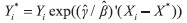 | (3) |
Notice that the expression (3) does not contain the scaling factors, which ensures that equivalent income, unlike subjective well-being score, does not depend on aspirations. Person i’s equivalent income is a function of her income, an ordinal preference (i.e. “pan-European”) determined by the ratios (  ) and of the shortfalls of her non-income dimensions from their best levels, ( Xi− X*). If Y’s are all zero (meaning that non-income dimensions do not affect subjective well-being at all) or if non-income dimensions are all at their best levels, then Y i*= Yi will hold. In all other cases Yi*< Yi will hold, depending on how strongly non-income dimensions are valued relative to income and how far they are from their best levels. Generally, the more (less) valued non-income dimensions are relative to income, and the larger (smaller) the gaps between the actual and best levels of non-income dimensions, the farther (closer) will equivalent income be from income.
The concept of equivalent income as we use it in this paper treats ordinal preferences as common to all individuals. In other words, there is no preference heterogeneity among individuals, not even among groups of individuals. In that respect our usage of the concept of equivalent income as a measure of multidimensional wellbeing differs from how it is originally motivated by Decancq, Fleurbaey and Schokkaert ( 2015a; 2015b) and applied by Schokkaert, Van Ootegem and Verhofstadt ( 2011), Decancq, Fleurbaey and Schokkaert ( 2015a; 2015b; 2016), Decancq and Schokkaert ( 2016), Decancq and Neumann ( 2016), Decancq, Schokkaert and Zuluaga ( 2016), Defloor, Verhofstadt and Van Ootegem ( 2017 ). They are primarily motivated by the possibility of taking into account heterogeneity of preferences. Not doing so would amount to neglecting the principle of individual sovereignty (or the “personal preference principle” in Decancq, Fleurbaey and Schokkaert’s ( 2015a; 2015b) terminology), an idea of individuals differing in what they themselves consider to be a good life. Put differently, respecting individual sovereignty means respecting differences in how people weight different life dimensions. In these papers, preference heterogeneity is modelled by introducing variables deemed relevant for differences in preferences, by way of interacting them with income and non-income dimensions in model (2). Since it is impossible to estimate strictly individual preferences, preference heterogeneity is modelled and estimated as heterogeneity among a number of social groups, depending on the choice of variables affecting preferences and the range of values or modalities of these variables. All the papers mentioned above found that there is preference heterogeneity.
The reason why we consider homogeneous, rather than heterogeneous, preferences relates to our objective to investigate changes in well-being and its distribution in the European Union over the period 2007-2011. We are focused on comparing well-being using income and equivalent income measures. If we opted for heterogeneous preferences, in accounting for changes over time we would need to distinguish between, on the one hand, the effect of changes in income and non-income dimensions and, on the other hand, the effect of changes in preferences. This task would be difficult without complicating the analysis and drawing attention away from our main objective, namely to explore the consequences of using a multi-dimensional well-being concept instead of income. 4 This is not to deny the potential importance of preference heterogeneity, but rather to simplify the analysis of a topic that is still scarcely researched.
3 Data
3.1 European Quality of Life Survey
The data we use come from the European Quality of Life Survey (EQLS) 2007 and 2011 for the EU-27 countries.6 For this study, it is important that the EQLS contains data on life satisfaction, income, a number of non-income dimensions and a sufficiently rich set of personal and household characteristics to be used as the scaling factors. The sample sizes differ across countries and years. The sample of all completed interviews ranges in 2007 from 1000 to 2008 and in 2011 from 1000 to 3055, with the mean sizes of respectively 1134 and 1315. After removing observations with incomplete information, we are left in 2007 with the range from 376 to 1364 and in 2011 from 474 to 2312, with the respective means of 700 and 930. The model (2) is thus estimated on the total sample of 44,016 observations (67 percent of the total original sample) consisting of 18,899 observations for 2007 and 25,117 observations for 2011. In appendix Table A1 we give the number of observations per country and year.
3.2 Variables: subjective well-being; income; non-income dimensions and scaling factors
3.2.1 Subjective well-being: life satisfaction
The variable representing it in the survey is the life satisfaction score, an integer on a 1-10 scale. It is the response to the question: All things considered, how satisfied would you say you are with your life these days? Please tell me on a scale of 1 to 10, where 1 means very dissatisfied and 10 means very satisfied.
3.2.2 Income
We rely on disposable household income per adult equivalent.7 The survey first asks for the household’s disposable income per month, and if the respondent does not know the exact amount, she can choose one among 21 income intervals. For those individuals who have answered the latter question only, the average of the interval’s limits is taken. All incomes are converted by Eurofound into purchasing power standard (PPS) euros. Since in our analysis we deal with the population means and inequality measures, it is important for us that these statistics, calculated from the EQLS income data, match as closely as possible those calculated from other sources, such as national accounts in the case of population mean and Eurostat’s figures on income inequality derived from the EU-SILC8.
To ensure that, we had to do rescaling of the EQLS incomes, the purpose of which is to ensure the following. First, the decile shares of equivalised household disposable income from the EQLS must be equal to the decile shares from the EU-SILC. Under the assumption that most inequality in income distribution is due to differences between the mean incomes of decile groups, by getting the decile income shares in line with those based on the EU-SILC income data we try to obtain Gini indices of income inequality computed from the EQLS incomes to be as close as possible to the Ginis computed from the EU-SILC incomes. Second, the mean disposable income per household member must be equal to the closest concept from national accounts in per capita terms. Following Decancq and Schokkaert ( 2016), we take that national accounts income concept to be the net national income per capita (obtained from Eurostat). 9
3.2.3 Non-income dimensions
Unemployment. A person is considered unemployed if he/she reported. Economic inactivity is clearly distinguished from unemployment, so that the retired, housewives and others outside of the labour market and not working are “non-unemployed.” Thus, the alternative to unemployment is not employment, but rather non-unemployment (of which employment is but one form). Research has shown that unemployment may be psychically harmful (e.g., Clark and Oswald, 1994; Darity and Goldsmith, 1996; Helliwell and Huang, 2014; Wulfgramm, 2014), and for that reason being unemployed is here considered an unfavourable status apart from its effect on the material living standard through income loss.
Health. Health is measured by the answers to the standard question on general selfassessment of one’s health. The answer modalities are very good, good, fair, bad and very bad. Yet, since this information about a person’s general health situation is necessarily the person’s subjective expression of her general feeling, one may object that it should not be used as indicating objective features of her state of health. The grounds for the objection would be the same as the grounds for arguing against using the subjective well-being score as a measure of well-being, namely that self-assessment of health is highly influenced by health aspirations, just as subjective well-being is influenced by general well-being aspirations. These aspirations are conceivably related to certain personal characteristics, such as age, sex and personal health history. However, there are studies showing that self-assessed health is indeed sufficiently strongly associated with mortality, even after controlling for potential confounders, such as depression and co-morbidity (for reviews, see Idler and Benyamini, 1997; Kawada, 2003 and DeSalvo et al., 2006).
Housing quality. The survey asks respondents if they have any of the following problems with their accommodation: i) shortage of space, ii) rot in windows, doors or floors, iii) damps or leaks in walls or roof, iv) lack of indoor flushing toilet and v) lack of bath or shower. An important reason why housing quality may not be redundant when income is included is that respondents are not asked to report their permanent income, a longer-term average, but rather the amount they command currently. That said, if the permanent income is low in spite of the current one being high, then given that improvements in housing quality usually require sizeable expenses (say, buying a new apartment or doing a major renovation), high current income can go along with low housing quality.
Crime. It has been shown that crime has an adverse effect on well-being (e.g., Powdthawee, 2005; Cornaglia, Feldman and Leigh, 2014; Dustmann and Fasani, 2016). The respondent is asked whether he/she has major, moderate or no problems with crime, violence or vandalism in the immediate neighbourhood of his/her home. People may care not only about crime, violence and vandalism in the immediate neighbourhood, but also in a wider area, presumably for fear of possible spillover effects on the narrow areas they live in. Yet, arguably, the situation with crime in people’s immediate neighbourhood is much more important for their well-being than the situation with crime in the country as a whole.
Environmental quality. Environmental quality covers the quality of drinking water and air. Thus, one’s possible concerns for the natural environment in general, with its many aspects, are not entirely captured, except insofar as the captured aspects are related to environmental problems in general. As in the case of crime, the focus is on problems with drinking water and air in one’s immediate neighbourhood, and not in the country as a whole. The survey question is also posed in the same way as in the case of crime: whether the respondent has major, moderate or no problems with drinking water and air pollution.
3.2.4 Scaling factors
The EQLS contains information on a rich set of socio-demographic characteristics and attitudinal variables. We use a number of these as the scaling factors: age, sex, education, marital/relationship status, settlement type (degree of urbanisation), parental status, and trust in people and institutions. These variables, together with some of the variables we take as well-being dimensions, are commonly used as covariates in life satisfaction and happiness regressions. Moreover, more often than not, many of them are usually found both substantially and statistically significant (Dolan, Peasgood and White, 2008).
Summary statistics for all variables (i.e. life satisfaction, dimensions and scaling factors) are given in Appendix Table A2.
4 Estimation of preferences and calculation of equivalent incomes
To estimate the parameters determining preferences, we specify the following model of life satisfaction: 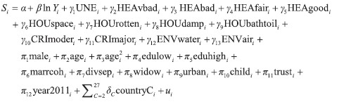 | (4) |
The estimates are presented in Table 1. We first estimated model (4) separately for each year. Coefficients determining preferences for 2007 are in general very similar to those for 2011 with only one statistically significant difference for the lack of bath or flushing toilet10. Thus, we have decided to pool the two years together for estimation. The results are generally in accordance with the existing literature estimating life satisfaction regressions (see Frey and Stutzer, 2002; Dolan, Peasgood and White, 2008 and Helliwell, Layard and Sachs, 2012).
Table 1Ordered logit estimation of life satisfaction model DISPLAY Table
All coefficients determining preferences have the expected signs, they are positive for income and negative for the indicators representing non-income dimensions. The coefficients on non-income dimensions are negative because for each of them the reference is the best level. All these coefficients are also statistically highly significant. Concerning the scaling factors, the signs of estimated coefficients are generally in line with the broad literature.
We plug the estimated preference parameters (β and Ɣ’s) in expression (3) to obtain each individual’s equivalent income. Since the most preferred levels of all indicators representing non-income dimensions are equal to zero, individual equivalent income is given by:  | (5) |
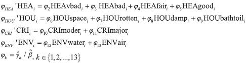
So far, we did not compare the magnitudes of the preference parameter estimates, as we have only commented on the signs of these estimates. To see how strong, the deprivations in non-income indicators are relative to each other, we do the comparison in the following way. We compute how large a person’s equivalent income relative to her income would be if she suffered just one particular deprivation. This gives us 13 different values of equivalent income expressed as a percentage of income. Comparing them with one another shows each indicator’s relative importance. In addition, since without any deprivation, equivalent income equals income, we can see just how harmful the shortfall in a particular non-income dimension from its best level is for individual multidimensional well-being.
These relative equivalent incomes are shown in Figure 1. What strikes one immediately is the importance of health, as those individuals with very bad, bad or fair, rather than very good health, have equivalent income as low as 0.1, 0.7 and 6.9 percent of their income, respectively. Equivalent income of the unemployed represents about 12 percent of their income. Those living in insufficiently spacious dwellings or dwellings with rotten parts see their well-being reduced by roughly 60 percent, while those facing damps or leaks and those living in neighbourhoods with major crime, violence or vandalism by about 50 percent of their income. Less harmful, but still notably so, is to have problems with the quality of drinking water or to have no bath or toilet, whose equivalent income is about two thirds of their income. Finally, those residing in neighbourhoods with moderate crime or vandalism and those with air quality problems suffer the least, as their equivalent incomes are below income by about a third and a quarter, respectively.
Figure 1Individual counterfactual equivalent income DISPLAY Figure
These magnitudes may seem unreasonable. Even if one accepts as reasonable that suffering from very bad or bad health is associated with very low well-being, the implied suffering of someone having good rather than very good health may seem quite exaggerated (about 75 percent of income). This intuition is based on what one would expect people to answer if asked directly in a contingent valuation; for example: "You consider your health good rather than very good. Suppose that you have the possibility to pay some percentage of your income to switch from good to very good health. What is this percentage?” Given problems with contingent valuation as a method of preference elicitation, it is not clear whether we need to take the average answer as a check of whether the percentages implied by preferences estimated through the life satisfaction approach are reasonable. Thus, even if many people considered the magnitudes of suffering from not attaining the best levels of non-income dimensions too high, this may not be sufficient to discard these magnitudes as unreasonable.
To check if the high magnitudes of suffering from deprivations in non-income dimensions are such only because of our data, it is useful to look at similar papers. For example, in a paper that also uses the life satisfaction approach to estimate preferences, Decancq and Schokkaert ( 2016) also estimated preference parameters that imply very high magnitudes of suffering from unemployment and less than perfect health. For example, their estimates imply that the equivalent income of a person with very bad health and no deprivations in other non-income dimensions is about one percent of her income, and the respective figures for bad, fair and good health are 4.2, 13.8 and 39 percent, respectively. As regards unemployment, an unemployed person’s equivalent income is about 11 percent of her income. 11
5 Income and equivalent income in the EU over 2007-2011
5.1 Average income and equivalent income
Levels of the average income (μ) and equivalent income (μ*) across countries and years are shown in Figure 2. There is a positive correlation between mean incomes and equivalent incomes: for levels, in 2007 (2011) it is 0.86 (0.96) while for ranks it is 0.95 for both years. Still, the rank for some countries changes substantially. For example, Italy in 2007 is ranked 13th by μ, and 19th by μ*, while Cyprus climbs from the 14th to the 7th place. However, for most countries the rank changes by only one or two places. This fact shows that taking non-income dimensions into account when constructing a well-being measure does not lead to a substantially different picture of how countries are ranked by the mean well-being.
Figure 2Average incomes and equivalent incomes DISPLAY Figure
In both years and for all countries, μ* amounts to less than half of μ or, in other words, the mean WTP amounts to more than half of the mean income. This shows that deprivations in non-income dimensions have a strongly detrimental effect on well-being, as expected given the effects of particular deprivations discussed in the previous section. Considering both years, the ratio μ*/μ (multiplied by 100) ranges from only 6.1 percent (Latvia in 2007) to 42.8 percent (Ireland in 2007), with the average of 20.4 percent in 2007 and 24.1 percent in 20 11. Further, the relative dispersion of μ is smaller than that of μ*. In 2007, the coefficient of variation (CV) of μ is 0.39, whereas for μ* we find CV = 0.64. The respective CVs for 2011 are 0.36 and 0.54. Thus, in relative terms, countries differ considerably less in their μ than in their μ*. This indicates that countries differ more from one another in terms of non-income dimensions than in terms of income, so that the relative differences in average well-being get amplified upon switching from income to equivalent income.
We turn now to the growth rates of μ and μ*. The bottom panel of Figure 2 shows the cumulative growth over 2007-2011. For all countries μ fell – expectedly, given the period studied. The drop in μ ranges from 2.9 percent in Poland to as much as 31.8 percent in Luxembourg and Greece, and for most of the countries (19 out of 27) the growth rates were in the range from -10 to -25 percent, with -17.3 percent on average. At this point, we have to stress that there are differences between these growth rates and the growth rates of GDP or even GDP per capita, for a number of reasons. First, individual income is rescaled for each country so that its mean per household member equals net national income per capita, and that its Gini coefficient comes as close as possible to the one reported by Eurostat. Second, the rescaled income is transformed from per-capita to per-adult-equivalent values. 12 Nevertheless, the growth rates have the same signs as the cumulative GDP growth rates over 2007-2011.
Was the growth performance so gloomy when we consider equivalent income, rather than income? Even at first glance, the growth rates of μ* hardly match those of μ. They are different not only in magnitude, but also in the sign. For about a half of the countries (14 out of 27), μ and μ* changed in opposite directions while for almost all of them, the increase in μ* is larger than the fall in μ. Growth rates of μ* range from -38.5 percent (Ireland) to 64.6 percent (Poland), with the average of 5.8 percent. Measured by the coefficient of variation, variation of growth in μ* is much higher (CV = 4.72) than variation of growth in μ (CV = 0.41). While we found a high positive correlation between μ and μ*, their growth rates are correlated much less, 0.42 (0.35) for growth levels (ranks). About a third of the countries change the rank by more than 10 places. Some extreme cases are Germany, the Netherlands and Cyprus, going 11, 12 and 16 places down, respectively; and on the other side Lithuania, Latvia and Italy, going 14, 15 and 17 places up, respectively. Thus, whereas the countries’ ranks by μ is very much in line with those by μ*, this hardly holds for their growth rates. Of course, this type of result may well depend on the period over which the growth rates are computed.
5.2 Income inequality and equivalent income inequality
As the inequality measure, we use the Atkinson index (Atkinson, 1970) with the inequality aversion parameter ε=1, A1, which ranges from zero (i.e. in case of perfect equality) to one (i.e. in case of perfect inequality): 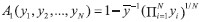 | (6) |
 is the mean income and N is the
population size. is the mean income and N is the
population size.
The Atkinson indices are shown in Figure 3. There is a striking difference between income and equivalent income inequality, the latter being much higher. While the Atkinson index for income (A1) ranges, depending on country and year, from 0.09 to 0.22, the index for equivalent income (A1*)13 is in the range 0.6-0.85. Considering both years, A1* is at least 3.5 times higher than A1 , and the ratio A1*/ A1 goes as high as 8, with the average of 5.3. Unlike in the case of means, where we had a high positive cross-country correlation, now the correlations are moderate with the level and rank correlations ranging between 0.60-0.66. Most of the countries change their rank by 6-8 places. The most extreme case is Hungary, with the fourth lowest A1 , but the second highest A1*, a jump of 21 places. Slovakia and Slovenia, in both years among the countries with lowest A1 , change their ranks substantially upon switching from income to equivalent income (Slovakia: 13 in 2007, 14 in 2011; Slovenia: 11 in both years). Thus, whereas high average income is a very good indication of high average equivalent income, high income inequality is a not-sogood indication of high equivalent income inequality.
Turning to changes in inequality over 2007-2011 we see that in most of the countries (16 out of 27) A1 was reduced, with the largest (relative) reduction in Belgium (18.2 percent), followed by Lithuania and Slovenia (about 13 percent). In most countries A1 fell by about 10 percent, and in only a few by less than 3 percent. Of the 11 countries with rising A1 , in seven of them the increase exceeded 10 percent, and in five it was close to or exceeded 20 percent (Denmark, Ireland, Greece, Czech Rep. and Hungary). The rise of more than 26 percent in Greece shows the economic slump had a very regressive distributive impact. Particularly remarkable increases took place in the Czech Republic where the Atkinson indeks went up by 39 percent, and in Hungary where it almost doubled (96 percent), though from relatively low levels.
Even a casual inspection reveals significant discrepancies between changes in A1 and A1*. The correlations are weak, 0.15 (0.36) for levels (ranks) of relative changes, both lower than the respective correlations between growth rates of the mean income and equivalent income. The directions of change are the same in only 16 countries, and mostly so for countries where inequality declined. While there are more countries with declining than with rising income inequality (declining in 16, rising in 11), the opposite holds in the case of equivalent income inequality (declining in 11, rising in 16). The magnitudes of changes also differ significantly. In almost all countries where changes are in the same direction, A1 changed more than A1*.
Figure 3Income and equivalent income inequality DISPLAY Figure
Thus, income and equivalent income inequalities do not need to change hand-inhand: they can differ in terms of the direction of change or magnitude. Clearly, in countries where income inequality declined, and equivalent income inequality increased, inequality-reducing changes in income distribution were outweighed by inequality-increasing changes in the distributions of (some) non-income dimensions. Take, for example, Malta, where A1 fell by 11.5 percent, whereas A1* increased by 4.9 percent. Similarly, where both income and equivalent income inequalities changed in the same direction, say increased, but the latter increases less (which, as the results show, tends to be the case), inequality-increasing changes in the income distribution took place along with inequality-reducing changes in the distributions of non-income dimensions. An example is the Czech Republic whose inequality in income increased by almost 40 percent, and inequality in equivalent income by about 5 percent only; or Hungary with almost doubled income inequality and virtually unchanged equivalent income inequality.
Given that equivalent income is a function of income, non-income dimensions and the parameters determining preferences (which are fixed), equivalent income inequality can come only from income inequality and inequality in non-income dimensions. We now explore the structure of equivalent income inequality by decomposing it into the respective contributions of inequalities in income and non-income dimensions. Unfortunately, such a decomposition cannot be done with the Atkinson index, so we need to use another measure of relative inequality, namely the variance of logarithms:14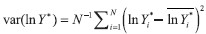 | (7) |
 is the mean of ɣ*i. is the mean of ɣ*i.
To do the decomposition, we first log-linearise equation (5) to get| lnYi* = lnYi + φ1UNEi + φ'HEAHEAi + φ'HOUHOUi +φ'CRICRIi +φ'ENVENV | (8) |
var(lnY*) = cov(lnY*, lnY) + cov(nY*, φ1UNE) + cov(lnY*, φ'HEAHEA) +
cov(lnY*, φHOUHOU) + cov(lnY*, φCRICRI) + cov(lnY*, φENVENV) | (9) |
The results are shown in Figure 4.15 In both years, the contribution of income is much smaller than that of non-income dimensions. In 2007 (2011), income contribution ranges from 8.1 (11.5) to 23.1 (19.7) percent, with the average of 14.3 (14.6) percent, while the rest can be attributed to non-income dimensions. Considering the contributions of non-income dimensions, health has by far the largest contribution, ranging in 2007 (2011) from 47.1 (47.6) to 70.7 (69.9) percent, with the average of 58.8 (58.8) percent. This is in accordance with the calculations in section 4, where we examined the relative importance of deprivations in each of the non-income dimension and saw that health is the most important (see Figure 1). The second largest contribution is that of housing, contributing 14.4 (12.6) percent on average in 2007 (2011). Then come unemployment, environment and crime. Note that the contribution of unemployment is the third largest despite the fact that it was the second most harmful individual non-income deprivation (see Figure 1). This is because here the extent of suffering from non-income deprivations at the societal level is taken into account, while the calculations in section 4 were done at the individual level.
Figure 4Decomposition of variance of logarithms of individual equivalent incomes DISPLAY Figure
5.3 Distribution-sensitive social welfare
Focusing on the means amounts to being concerned with the efficiency aspect of social welfare, while focusing on inequality amounts to being concerned with its equity aspect. However, one may be concerned with both aspects, and thus use a social welfare indicator capturing both. For that purpose, we use a social welfare function from the so-called Atkinson-Kolm-Sen class (Atkinson, 1970; Kolm, 1966; 1976; Sen, 1973). A general social welfare function from this class takes the form of the product between the mean income (or other well-being metric of interest) and a distributional “correction factor” equal to one minus the scalar inequality index chosen. As in the previous section, we use the Atkinson inequality indeks with the inequality aversion parameter ε=1. Thus, the income- and equivalent income-based social welfare functions are W=μ(1−A1) and W*=μ*(1−A1*), respectively. We chose this particular social welfare function because its relative change over time can be straightforwardly decomposed into the respective contributions of income changes and changes in non-income dimensions. 16 Yet besides this important property, the social welfare function has an appealing normative property as well, at least to those who care about the equity aspect of social welfare and at the same time do not have extreme inequality aversion. It can be shown that the marginal social weight of a person implied by this social welfare function monotonically decreases as one moves from the bottom to the top of the distribution. Precisely, the marginal social weight of person i with income Yi is 1/ Yi. Since this person’s contribution to social welfare is the product of her marginal social weight and her income, her contribution is (1/ Yi)· Yi=1, as it is for every other person. In contrast, for the social welfare function that does not take into account the equity aspect, which is the case if it is equated with the mean income, W=μ, a person’s marginal social weight is equal to her income. Therefore, while W=μ(1− A1) embodies the “one person, one vote” principle, W=μ embodies the “one euro, one vote” principle. In that sense, the former can be called “democratic”. This carries over to the evaluation of growth in social welfare, while in the case of the “democratic” social welfare function everyone’s growth is weighted equally in computing the overall growth, in the case of mean growth the weights are equal to incomes.
We first look at how much variations in means and inequality levels contribute to the cross-country variation in income- and equivalent income-based social welfare. We log-linearize W and W*, and then decompose the variance of ln W (ln W*) into the respective contributions of variations in lnμ (ln μ*) and variations in ln(1- A1) (ln(1- A*1)). In the case of income-based social welfare, we have | var(lnW) = cov(lnμ,lnW) + cov(ln(1-A1),lnW) | (10) |
for levels and | var(Δ lnW) = cov(ΔlnW,Δlnμ) + cov(ΔlnW,Δln(1-A1)) | (11) |
for changes, while the corresponding expressions for equivalent income-based social welfare are obtained by replacing ( W, μ, A1) with (W*, μ*, A1*). The first term on the right-hand side of (10) is the contribution of cross-country variation in the mean, while the second one is the contribution of variation in the inequality-correction factor. Analogously, in (11) the contributions correspond to changes.
Decomposition results are shown in Table 2. The variance in ln W is almost entirely accounted for by variation in ln μ, with contributions of 94.5 (93.5) percent in 2007 (2011), respectively. Thus, countries differ much more in their mean incomes than in inequality. Variance of ln W* is also predominantly explained by variation in ln μ*, but less so than in the case of income-based social welfare: the contribution is 75.6 (71.2) percent in 2007 (2011). These results indicate that in cross-country comparisons of social welfare, the failure to take into account inequality differences is more important when individual well-being is measured by equivalent income. If one deems the equity aspect of social welfare important, then one should be more concerned with it when social welfare is based on equivalent income; that is, when well-being is measured multi-dimensionally. The following result comes from negative correlation between income and deprivations in non-income dimensions where on average, higher income is associated with better non-income dimensions, both among individuals and countries. Regarding the variance of growth in social welfare, the results are similar for income- and equivalent income-based social welfare.
Table 2Decomposition of cross-country variance of levels and changes in social welfare DISPLAY Table
Income- and equivalent income-based social welfare are functionally related to each other. Taking the expected value of equation (8) for each country c∈{1, 2, ...,27}and year t∈{2007, 2011}, and noting that for inequality aversion parameter ɛ=1 it holds that E(ln Y*) c,t= ln W*c,t and E(ln Y) c,t= ln Wc,t we obtain 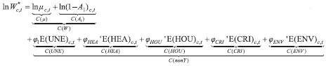 | (12) |
The corresponding expression for growth in equivalent income-based social welfare, Δln W*c, is obtained by subtracting (12) between two years, whereby the C(X) terms turn into C(Δ X). By definition, C( μ) contributes positively, while C( A1), C( UNE), C( HEA), C( HOU), C( CRI) and C( ENV) contribute negatively to ln W*c,t. Here we are interested in how the cross-country variations in ln W*c,t and Δln W*c are accounted for by the respective variations in their constitutive elements. For the purpose, we again use variance decomposition.
The results of variance decompositions are shown in Table 3. In both 2007 and 2011 the contribution of variation in non-income dimensions is larger than the contribution of variation in income-based social welfare, 60.7 vs. 39.3 (54.8 vs. 45.2) percent in 2007 (2011). Thus, if one is interested in cross-country differences in multidimensional and inequality-adjusted social welfare, one would miss a great deal by supposing that using only income-based social welfare amounts to using a good enough proxy. Such a practice may be reasonable if most of the variation in equivalent income-based social welfare were accounted for by the variation in income-based social welfare, which is not the case here. Omitting non-income dimensions would thus amount to neglecting a substantial, indeed dominant part.
Table 3Variance decomposition of equivalent income-based social welfare DISPLAY Table
Detailed decompositions reveal first that the contribution of income-based social welfare consists almost entirely of the contribution of mean income, a result in line with what we found earlier in this section. Regarding non-income dimensions, slightly more than half of their total contribution is due to health (31.4(31.1) percent in 2007 (2011)). The contribution of housing comes as the second most important non-income dimension, with a contribution of about half that of health. Then come environment, crime and, the least important, unemployment. What these results indicate is that health is a non-income dimension that certainly should not be left out. Variations in income-based social welfare and health account for about 75 percent of the total variation in equivalent-income based social welfare. Adding housing, the proportion accounted for to about 85 percent. Thus, considering only two non-income dimensions along with income goes a long way to account for cross-country variation in equivalent income-based social welfare, above what can be accounted for by income-based social welfare only.
In Figure 5 we show how changes in income-based social welfare and non-income dimensions contributed to changes in equivalent income-based social welfare. The contribution of growth in income-based social welfare is negative for all countries, since the negative growth in mean income was nowhere fully offset by inequality reduction (see Table 3). With some exceptions, the sign of changes in non-income dimensions determines the sign of growth in equivalent incomebased social welfare. Therefore, in countries where equivalent income-based social welfare increased, it did so due to improvements in non-income dimensions. 17 Moreover, in countries where non-income dimensions worsened, this reinforced the negative growth in income-based social welfare. The detailed decomposition reveals that the sign of the total contribution of non-income dimensions tends to match the sign of health contribution, underlining the importance of health. In all but one country unemployment worsened and thus contributed negatively, while in most countries there were improvements in housing, crime and environment, as evidenced by their mostly positive contributions.
Figure 5Decomposition of growth in equivalent income-based social welfare DISPLAY Figure
Considering the contributions to the variation of changes in equivalent income-based social welfare, 87.3 percent of the cross-country variance is accounted for by the contribution of non-income dimensions (see Table 3). These results clearly testify to the importance of considering non-income dimensions. By far the largest contribution is that of health, followed by the contributions of environment, crime, housing and unemployment. Thus, the combination of health and environment, accounts for more than 60 percent of the total contribution of non-income dimensions.
6 Summary and conclusions
The objective of this paper was to explore empirically how well-being comparisons among countries at a point in time and over time depend on two different concepts of individual well-being. Using individual survey data for 2007 and 2011 for 27 EU countries, we compared results based on multidimensional well-being measured by equivalent income with those based on equating individual wellbeing with income. In constructing equivalent income, we combined income with five non-income dimensions, namely unemployment, health, housing, crime and environment. The relative weights of income and non-income dimensions are based on estimated “pan-European” preferences. We have made cross-country comparisons not only in terms of the average levels of income and equivalent income, but also in terms of inequality in their respective distributions and in terms of social welfare capturing both the averages (efficiency aspect) and inequality levels (equity aspect).
Our results and their implications can be summarised as follows. The ranking of countries in a given year by the mean equivalent income is very much in accordance with the ranking by mean income. Therefore, if one is interested in crosscountry comparisons of the average well-being levels at a point in time, one hardly gets anything new upon switching from income to equivalent income. However, although the rankings are similar, the relative dispersion of mean equivalent incomes is considerably larger than that of mean incomes, indicating that countries are more similar to each other in terms of income than in terms of nonincome dimensions. While the rankings by the means are very similar, this hardly holds for their growth rates. Not only the magnitudes of the growth rates but also their signs are different (i.e. some countries experienced an increase in mean income and decrease in mean equivalent income over the same period).
Equivalent income inequality is substantially higher than income inequality, a consequence of the income gradient of non-income dimensions and high sensitivity of equivalent income to shortfalls of certain non-income dimensions from their most favourable levels, especially in the cases of health and unemployment. Distributional issues are thus much more important when individual well-being is measured by equivalent income. Decompositions of equivalent income inequality reveal that in all countries the single largest contribution is that of variation in health status.
The ranking of countries by equivalent income inequality in a given year is substantially different from the ranking by income inequality. Thus, while the use of equivalent income instead of income hardly changes cross-country comparisons of the average level of well-being, comparisons of inequality levels change a great deal. This conclusion holds even more for cross-country comparisons of changes in inequality since there is only a weak correlation between percentage changes in equivalent income inequality and changes in income inequality.
Comparing countries in terms of social welfare by means of a social welfare function that captures both aspects of efficiency and equity is much more important when well-being is measured by equivalent income. Whereas income-based social welfare varies across countries almost entirely due to variation in the mean income, in the case of equivalent income-based social welfare the contribution of variation in equivalent income inequality is far from negligible. Therefore, considering equity when assessing social welfare is more important when individual well-being is measured by equivalent income.
Cross-country variation in equivalent income-based social welfare is more accounted for by variation in average levels of non-income dimensions than by variation in average income and income inequality. The contribution of health comes out as by far the most important. Leaving out non-income dimensions, especially health, would be to leave unexplained more than half of the crosscountry variation in equivalent income-based social welfare. In accounting for the cross-country variation in growth of equivalent income-based social welfare, the contribution of variation in non-income dimensions is even more important. This indicates that ignoring non-income dimensions is more important for explaining differences in growth than in levels of equivalent income-based social welfare.
We see these results as providing evidence that it matters a great deal whether we look at well-being and its distribution through the unidimensional lenses of someone committed to taking income as individual well-being measure or through multidimensional lenses of someone who acknowledges the importance of going beyond income by considering non-income dimensions as well. We conclude that by disregarding non-income dimensions, and health in particular, and focusing solely on income, one effectively leaves a great deal of well-being differences – both among individuals and among countries –unexplained. The unidimensional picture of well-being painted by income is in many respects different from the multi-dimensional picture painted by equivalent income.
Appendix
Table A1Number of observations per country and year DISPLAY Table Table A2Variable definitions and summary statistics DISPLAY Table
Appendix 2
The rescaling procedure proceeds in four steps. First, using the Eurostat data on the decile shares in aggregate equivalized (by the OECD scale) disposable income and the mean equivalized disposable income, we calculate, for each country-year, the mean for each decile group, μd, using the fact that μd=sdμ, where sd is the decile share, and μ is the overall mean. In the second step, we divide the decile means μd by the corresponding decile means calculated from the EQLS data to obtain decilespecific rescaling factors for each country-year. Then we multiply all incomes in each of the EQLS decile groups for each country-year by the corresponding rescaling factors, to ensure that for each country-year the decile shares from the EQLS data are equal to those from the Eurostat data. Third, from the rescaled equivalized incomes, we recover the total rescaled household incomes, from which we calculate rescaled disposable household incomes per household member (rather than per adult equivalent). These are further rescaled by multiplying them by country-yearspecific rescaling factors obtained as the ratio of the net national income (NNI) per capita (in purchasing power standard) to the mean disposable household income per household member. This ensures equality, between the NNI per capita and the mean disposable household income per household member. In the last step, we calculate new total disposable household incomes and divide them by the number of adult equivalents to obtain the disposable household income per adult equivalent. Finally, to convert nominal to real incomes, we divide them all by country-year specific consumer price indices (with 2005 as the base year). The income variable so obtained is the one we use in the analysis.
Upon applying the procedure, we have checked if the Gini coefficients calculated from the rescaled EQLS incomes match those obtained from Eurostat and found that almost all of the initial differences vanish (Figure A1). There is a concern that the rescaling distorts the original incomes too much, in the sense that the rescaling leads to substantial reranking among individuals (person A has higher income than person B before rescaling, but lower after rescaling). We computed the portion of the difference between the Gini coefficients for the original and rescaled incomes that can be attributed to reranking. We did that by performing the decomposition: Go˗Gr=(Go˗Cr)+(Cr˗Gr) where Go is the Gini coefficient for the original incomes, Gr is the Gini coefficient for the rescaled incomes and Cr is the concentration index for the rescaled incomes with respect to the original incomes. The term (Cr˗Gr) measures the reranking caused by the rescaling and we found that it is very small relative to the difference (Go˗Gr) (Figure A2), meaning that the rescaling spreads the income distribution without causing much reranking. We consider that a good enough indication that the rescaled incomes are not distorted too much and are thus reliable. Results are available on request. The more so given that not all respondents report the exact household income, but rather choose one of 21 intervals.
Figure A1Gini coefficients for original and rescaled incomes DISPLAY Figure
Figure A2Decomposition of the difference between the Gini coefficient for original and rescaled incomes DISPLAY Figure
Notes
* The authors would like to thank the two independent reviewers for their most useful suggestions and comments.
1 Countries (abbreviations) are: Austria (AT), Belgium (BE), Bulgaria (BG), Cyprus (CY), Czech Republic (CZ), Germany (DE), Denmark (DK), Estonia (EE), Greece (EL), Spain (ES), Finland (FI), France (FR), Hungary (HU), Ireland (IE), Italy (IT), Lithuania (LT), Luxembourg (LU), Latvia (LV), Malta (MT), Netherlands (NL), Poland (PL), Portugal (PT), Romania (RO), Sweden (SE), Slovenia (SI), Slovakia (SK), United Kingdom (UK). The abbreviations will be used in figures throughout the paper.
2 Of the current EU member states, only Croatia is left out, as it was not yet a member state during in this period.
3 Research has shown that the answers to these two types of question in existing surveys are highly correlated (Clark, 2016), more than the conceptual distinction would suggest.
4 Using the terminology from Decancq, Fleurbaey and Schokkaert (2015a; 2015b) and Decancq and Schokkaert (2016).
5 Decancq and Schokkaert (2016) argue that interpreting changes in equivalent income over time becomes difficult if one wants to retain the heterogeneity of preferences.
6 See link.
7 Based on the OECD equivalence scale: the first adult is counted as 1, the remaining adults as 0.5 each, and children as 0.3 each, where children are household members aged 0-13 years.
8 European Union Statistics on Income and Living Conditions – the official source of distributional statistics for the European Union of Eurostat.
9 The rescaling procedure is described in Online-Appendix. We also provide a comparison of inequality measures for incomes before and after rescaling and, in addition, analyse how much incomes are distorted by the recaling.
10 According to the Chow test.
11 Unlike our model, Decancq and Schokkaert's (2016) model of life satisfaction allows for preference heterogeneity and non-linearity of income and health effects on life satisfaction. The figures we report are based on preferences of their reference group, but those for other groups do not differ very much, and thus generally imply strong suffering from deprivations in non-income dimensions as well. The model is estimated on the 2008 and 2010 European Social Survey data for 18 countries. The reason for choosing this paper for comparison is that other papers estimate preferences for single countries and thus may not be comparable (Decancq, Fleurbaey and Schokkaert,2015a; 2017; Decancq and Neumann, 2016; Decancq, Schokkaert and Zuluaga, 2016). However, even the estimates from these papers imply very high suffering from deprivations in non-income dimensions, of the order of magnitude estimated in the present paper.
12 For details, see the data section and Online Appendix.
13 The Atkinson index for equivalent income should not be confused with Tsui’s (1995) generalisation of this inequality measure to the multidimensional context.
14 We checked the correlation between the variance of logarithms of income/equivalent income and the Atkinson index that we used. The correlations are quite high. In the case of income, the level (rank) correlation is 0.96 (0.96) in 2007 and 0.76 (0.89) in 2011. In the case of equivalent income, the level (rank) correlation is 0.93 (0.92) in 2007 and 0.95 (0.95) in 2011.
15 We divide equation (9) by var(ln Y*) and multiply it by 100 to get the contributions add up to 100.
16 This decomposition is shown below in this section; see equation (12).
17 Precisely, net improvements, since not all non-income dimensions necessarily improved.
* The authors would like to thank the two independent reviewers for their most useful suggestions and comments.
1 Countries (abbreviations) are: Austria (AT), Belgium (BE), Bulgaria (BG), Cyprus (CY), Czech Republic (CZ), Germany (DE), Denmark (DK), Estonia (EE), Greece (EL), Spain (ES), Finland (FI), France (FR), Hungary (HU), Ireland (IE), Italy (IT), Lithuania (LT), Luxembourg (LU), Latvia (LV), Malta (MT), Netherlands (NL), Poland (PL), Portugal (PT), Romania (RO), Sweden (SE), Slovenia (SI), Slovakia (SK), United Kingdom (UK). The abbreviations will be used in figures throughout the paper.
2 Of the current EU member states, only Croatia is left out, as it was not yet a member state during in this period.
3 Research has shown that the answers to these two types of question in existing surveys are highly correlated (Clark, 2016), more than the conceptual distinction would suggest.
4 Using the terminology from Decancq, Fleurbaey and Schokkaert ( 2015a; 2015b) and Decancq and Schokkaert ( 2016).
5 Decancq and Schokkaert ( 2016) argue that interpreting changes in equivalent income over time becomes difficult if one wants to retain the heterogeneity of preferences.
7 Based on the OECD equivalence scale: the first adult is counted as 1, the remaining adults as 0.5 each, and children as 0.3 each, where children are household members aged 0-13 years.
8 European Union Statistics on Income and Living Conditions – the official source of distributional statistics for the European Union of Eurostat.
9 The rescaling procedure is described in Online-Appendix. We also provide a comparison of inequality measures for incomes before and after rescaling and, in addition, analyse how much incomes are distorted by the recaling.
10 According to the Chow test.
11 Unlike our model, Decancq and Schokkaert's ( 2016) model of life satisfaction allows for preference heterogeneity and non-linearity of income and health effects on life satisfaction. The figures we report are based on preferences of their reference group, but those for other groups do not differ very much, and thus generally imply strong suffering from deprivations in non-income dimensions as well. The model is estimated on the 2008 and 2010 European Social Survey data for 18 countries. The reason for choosing this paper for comparison is that other papers estimate preferences for single countries and thus may not be comparable (Decancq, Fleurbaey and Schokkaert, 2015a; 2017; Decancq and Neumann, 2016; Decancq, Schokkaert and Zuluaga, 2016). However, even the estimates from these papers imply very high suffering from deprivations in non-income dimensions, of the order of magnitude estimated in the present paper.
12 For details, see the data section and Online Appendix.
13 The Atkinson index for equivalent income should not be confused with Tsui’s ( 1995) generalisation of this inequality measure to the multidimensional context.
14 We checked the correlation between the variance of logarithms of income/equivalent income and the Atkinson index that we used. The correlations are quite high. In the case of income, the level (rank) correlation is 0.96 (0.96) in 2007 and 0.76 (0.89) in 2011. In the case of equivalent income, the level (rank) correlation is 0.93 (0.92) in 2007 and 0.95 (0.95) in 2011.
15 We divide equation (9) by var(ln Y*) and multiply it by 100 to get the contributions add up to 100.
16 This decomposition is shown below in this section; see equation (12).
17 Precisely, net improvements, since not all non-income dimensions necessarily improved.
Disclosure statement
No potential conflict of interest was reported by the authors.
References
Atkinson, A. B.,1970. On the measurement of inequality. Journal of Economic Theory, 2(3), pp. 244–263.
Bache, I., 2013. Measuring quality of life for public policy: An idea whose time has come? Agenda-setting dynamics in the European Union. Journal of European Public Policy, 20(1), pp. 21–38 [ CrossRef]
Clark, A. E. and Oswald, A. J., 1994. Unhappiness and unemployment. Economic Journal, 104(424), pp. 648–659.
Clark, A. E., 2016. SWB as a measure of individual well-being. In M. Adler and M. Fleurbaey, eds. Oxford Handbook of Well-Being and Public Policy, pp. 518–552 [ CrossRef]
Cornaglia F., Feldman, N. E. and Leigh, A., 2014. Crime and mental well-being. Journal of Human Resources, 49(1), pp. 110–140.
Darity Jr., W. and Goldsmith, A. H., 1996. Social psychology, unemployment and macroeconomics. Journal of Economic Perspectives, 10(1), pp. 121–140 [ CrossRef]
Decancq, K. and Neumann, D., 2016. Does the choice of well-being measure matter empirically? In: M. Adler and M. Fleurbaey, eds. Oxford Handbook of Well-Being and Public Policy. Oxford: Oxford University Press [ CrossRef]
Decancq, K. and Schokkaert, E., 2016. Beyond GDP: using equivalent incomes to measure well-being in Europe. Social Indicators Research, 126(1), pp. 21–55 [ CrossRef]
Decancq, K., Fleurbaey, M. and Schokkaert, E., 2015a. Happiness, equivalent income and respect for individual preferences. Economica, 82(s1), pp. 1082–1106 [ CrossRef]
Decancq, K., Fleurbaey, M. and Schokkaert, E., 2015b. Inequality, income, and well-being. In: A. B. Atkinson and F. Bourguignon F., eds. Handbook on Income Distribution, vol. 2, pp. 67–140 [ CrossRef]
Decancq, K., Fleurbaey, M. and Schokkaert, E., 2017. Well-being inequality and preference heterogeneity. Economica, 84(334), pp. 210–238 [ CrossRef]
Decancq, K., Schokkaert, E. and Zuluaga, B., 2016. Implementing the capability approach with respect for individual valuations: an illustration with Colombian data. CORE Discussion Papers, 2016/36 [ CrossRef]
Defloor, B., Verhofstadt, E. and Van Ootegem, L., 2017. The influence of preference information on equivalent income. Social Indicators Research, 131(2), pp. 489–507 [ CrossRef]
DeSalvo, K. B. [et al.], 2006. Mortality prediction with a single general self-rated health question. Journal of General Internal Medicine, 20(3), pp. 267–275 [ CrossRef]
Dolan, P., Peasgood, T. and White, M., 2008. Do we really know what makes us happy? A review of the economic literature on the factors associated with subjective well-being. Journal of Economic Psychology, 29(1), pp. 94–122 [ CrossRef]
Dustman, C. and Fasani, F., 2016. The effect of local area crime on mental health. Economic Journal, 126(539), pp. 978–1017 [ CrossRef]
Fleurbaey, M. [et al.], 2012. Equivalent income and fair evaluation of health care. Health Economics, 22(6), pp. 711–729 [ CrossRef]
Fleurbaey, M. and Gaulier, G., 2009. International comparisons of living standards by equivalent incomes. Scandinavian Journal of Economics, 111(3), pp. 529–624 [ CrossRef]
Fleurbaey, M., 2015. Beyond income and wealth. Review of Income and Wealth, 61(2), pp. 199–219 [ CrossRef]
Frey, B. S. and Stutzer, A., 2002. Happiness and economics. Princeton: Princeton University Press.
Helliwell, J. and Huang, H., 2014. New measures of the cost of unemployment: evidence from the subjective well-being of 3.3 million Americans. Economic Inquiry, 52(4), pp. 1485–1502 [ CrossRef]
Helliwell, J., Layard, R. and Sachs, J., 2012. World happiness report. The Earth Institute, Columbia University.
Idler, E. L. and Benyamini, Y., 1997. Self-rated health and mortality: A review of twenty-seven community studies. Journal of Health and Social Behavior, 38(1), pp. 21–37 [ CrossRef]
Jara, H. X. and Schokkaert, E., 2016. Putting subjective well-being to use for ex-ante policy evaluation. EUROMOD Working Paper Series, EM 9/16 [ CrossRef]
Jones, C. I. and Klenow, P. J., 2017. Beyond GDP? Welfare across countries and time. American Economic Review, 106(9), pp. 2426–2457 [ CrossRef]
Kawada, T., 2003. Self-rated health and life prognosis. Archives of Medical Research, 34(4), pp. 343–347 [ CrossRef]
Kolm, S.-C., 1966. The optimal production of social justice. In: Colloques Internationaux du Centre National de la Recherche Scientifique. Biarritz, pp. 2–9.
Kolm, S.-C., 1976. Unequal inequalities I. Journal of Economic Theory, 12, pp. 416–442.
Ledić, M. and Rubil, I., 2019. Decomposing the Difference Between Well-Being Inequality and Income Inequality: Method and Application In: K. Decancq and P. Kerm, eds. What Drives Inequality? Research on Economic Inequality, 27, pp. 105–122 [ CrossRef]
OECD, 2011. How's life? Meausuring well-being. Paris: OECD.
Powdthavee, N., 2005. Unhappiness and crime: Evidence from South Africa. Economica, 72(287), pp. 531–547 [ CrossRef]
Samson, A.-L. [et al.], 2017. Fairness in cost-benefit analysis: A methodology for health technology assessment. Health Economics, 27(1), pp. 102–114 [ CrossRef]
Schokkaert, E., Van Ootegem, L. and Verhofstadt, E., 2011. Preferences and Subjective Satisfaction: Measuring Well-being on the Job for Policy Evaluation. Cesifo Economic Studies, 57(4),pp. 683–714.
Schokkaert, E. [et al.], 2013. Equity in health and equivalent incomes. Research on Economic Inequality, 21, pp. 131–156 [ CrossRef]
Sen, A. K., 1973. On economic inequality. Oxford: Clarendon Press.
Sen, A. K., 1985. Commodities and capabilities. Oxford: Oxford University Press.
Stiglitz, J. E., Sen, A. K. and Fitoussi, J.-P., 2010. Mismeasuring our lives: Why GDP doesn't add up. New York: The New Press.
Tsui, K. Y., 1995. Multidimensional Generalizations of the Relative and Absolute Inequality Indices: The Atkinson-Kolm-Sen Approach. J ournal of Economic Theory, 67(1), 251–265 [ CrossRef]
Wulfgramm, M., 2014. Life satisfaction effects of unemployment in Europe: The moderating influence of labour market policy. Journal of European Social Policy, 24(3), pp. 258–272 [ CrossRef]
|


