|
|
|
Abstract
This paper analyzes fiscal convergence and sustainability in the European Union using data on government debt, revenues, and expenditures. Absolute fiscal divergence is present in the EU, especially after the sovereign debt crisis. However, we find evidence of fiscal club convergence when clubs are endogenously determined. Club convergence is important for the EU because there is no single fiscal policy and member states’ policies are heterogeneous. Endogenous clubs do not share the usual geographical, political, or development similarities. Fiscal policy in the EU is found to be unsustainable, but it is countercyclical. We use a policy response function where the primary surplus is a function of public debt and the output gap. The primary surplus does not respond to changes in public debt, and this is considered to be unsustainable. However, it increases in expansions and decreases in recessions thus being countercyclical. The countercyclical primary surplus is important for smoothing business cycles.
Keywords: convergence clubs; fiscal sustainability; public debt; structural breaks; log t test; dynamic panel
JEL: C32, C33, E62, H60
1 Introduction
With the sovereign debt crisis in the Eurozone, fiscal policy has become an increasingly important topic. The sovereign debt crisis and the Great Recession led to many European Union countries breaching the public debt and deficit goals set by Stability and Growth Pact (SGP). The goals are for public debt not to exceed 60% of GDP and for the deficit not to exceed 3% of GDP. These goals, which are part of the nominal convergence criteria, were established to ensure sound and sustainable public finances in the European Union. However, whether or not there is a convergence of member states’ fiscal policies and whether fiscal policy is sustainable is still an open question.
This paper analyzes fiscal convergence and tests for fiscal sustainability in the European Union. We test fiscal convergence directly using government revenue, expenditure, and debt as key government variables instead of testing for GDP convergence as is usual in the convergence literature. The paper considers both absolute convergence and convergence clubs, which is important because the European Union does not have a single fiscal policy and member states’ policies are heterogeneous. Heterogeneous fiscal policies among member states could easily lead to different fiscal convergence clubs, which are analyzed in the paper. Based on the identified convergence clubs, we test for fiscal sustainability in the clubs as well as in the whole of the European Union. Fiscal sustainability has become an especially important topic for the EU countries after the Greek crisis.
The literature on fiscal convergence is relatively scarce. Economic integration, common institutional factors, and common policies in the EU should lead to convergence in key fiscal indicators. On the other hand, the sovereign debt crisis and the Great Recession affected member states in different ways, possibly leading to fiscal divergence. It seems that the observed period plays an important role. Earlier research finds some evidence of fiscal convergence in the period from the late 1960s to the early 2000s (De Bandt and Mongelli,  2000 2000; and Delgado, 2006), while more recent studies such as Kočenda, Kutan and Yigit ( 2008) show the lack of it in the period from 1995 to 2005. The mentioned papers measure convergence using the popular β- and α-convergence tests as well as cointegration tests in a time series framework.
The literature does not tackle the issue of convergence clubs regarding fiscal policy. However, the idea of convergence clubs is implicitly included in discussions on the EU core and periphery, or on the two-speed Europe idea popularized by Blanchard ( 2010) which argues that different groups of European countries show faster and slower recoveries after the Great Recession. Accordingly, fiscal convergence and the possibility of convergence clubs are important issues for EU policymakers. This paper analyzes both absolute convergence and club convergence. Instead of grouping countries according to ad-hoc criteria such as geographical location or EU accession date, we determine convergence clubs endogenously.
We also analyze fiscal sustainability within the clubs and in the whole EU 28 using a policy response function proposed by Bohn ( 1998; 2007). Fiscal policy is sustainable if the primary government surplus increases as a response to the increase in public debt. This is considered responsible and sustainable behavior because the government increases its revenue or decreases spending when faced with a higher public debt. Bohn (( 1998; 2005) concludes that U.S. fiscal policy is sustainable. Cassou, Shadmani and Vázquez ( 2017) refine this finding by showing that the U.S. fiscal policy is sustainable only during good economic times, but not in times of economic distress.
The research regarding European fiscal policy is somewhat different. Collignon ( 2012) develops a policy response function to analyze European fiscal sustainability. His policy response function is adjusted to EU fiscal rules looking at the primary surplus response to changes in debt and deficit. Results indicate that European fiscal policy is sustainable in this respect, but conditions on financial markets and the risk of financial contagion can make it insufficient, as shown by the Greek crisis. Research has also focused on the cyclical behavior of fiscal policy. The common understanding is that fiscal policy should be countercyclical; higher government spending in recessions followed by fiscal consolidation in expansions to smooth business cycles. The countercyclical fiscal policy is sustainable in the long run when extra deficits accumulated in recessions are compensated for during times of economic growth. Balassone, Francese and Zotteri ( 2010) show that budget balance in fourteen EU countries deteriorates during recessions, but does not improve to the same extent during expansions. Government expenditures are responsible for the asymmetry.
Public debt sustainability has been widely analyzed for individual countries as well. Babić ( 2003) and Mihaljek ( 2003) analyze the sustainability of public and external debt in Croatia. This early analysis 1 concluded that Croatian public debt is not too sensitive to the various shocks analyzed, but credit rating and interest rate spread in Croatia are worse than those of central European countries. Deskar Škrbić and Šimović ( 2017) on the other hand showed that public debt level affects the effectiveness of fiscal spending by reducing the size of fiscal effects in Croatia.
This paper contributes to the literature by analyzing absolute fiscal convergence and convergence clubs using quarterly data for government debt, revenues, and expenditures in EU member states from 2000:1 to 2017:2. We test convergence using a log t test proposed by Phillips and Sul ( 2007; 2009) accompanied with the clustering algorithm for endogenous club classification. Commonly used β- and σ-convergence tests might be biased and suffer from low power as noted in Bernard and Durlauf ( 1995; 1996) among others. Such tests assume linear dynamics in the convergence process. Phillips and Sul’s ( 2007) log t test is based on a nonlinear dynamic factor model, which allows a nonlinear adjustment in parameters both over time and across different countries. Therefore, it is suitable in testing for convergence. We check the robustness of our results by applying recently developed unit root tests, which control for both sharp and smooth structural breaks.
The paper also contributes to the fiscal policy sustainability literature. We use a policy response function proposed by Bohn ( 1998) in a panel framework where the primary government surplus is a function of public debt and the output gap. We use a dynamic panel model and include a lagged dependent variable in the equation since there is a strong inter-temporal relationship between the government surplus and public debt. Furthermore, EU countries are somewhat homogenous, and therefore there is a possibility of cross-sectional dependence. Unlike the previous literature, we use a dynamic panel system GMM estimator with common correlated effects proposed by Pesaran ( 2006) which controls for pronounced homogeneity among the EU countries.
The main findings can be summarized as follows. There is strong and robust evidence of absolute divergence in government debt, revenues, and expenditures among the EU countries. The process of divergence was intensified during the sovereign debt crisis and the Great Recession. However, we find two, three, and four endogenous convergence clubs in government debt, revenue, and expenditures respectively. The clubs are found to be quite heterogeneous; club members do not share the usual geographical, political, or development similarities. On the other hand, groups of EU-15 and EU-13 countries as well as EU core and EU periphery countries are shown to diverge, which suggests an important difference between endogenous and exogenous groupings.
Fiscal policy is found to be unsustainable but countercyclical both in the EU as a whole and within identified convergence clubs. Our model does not show an increase in the primary surplus after debt upsurge, which is identified as unsustainable behavior. We find only limited evidence of fiscal sustainability in the EU-13 group and in a subsample with public debt higher than 90%. On the other hand, fiscal policy in the EU is countercyclical, indicating the efforts of fiscal policy to smooth business cycles.
The paper is structured as follows. Section 2 explains and presents the data. It describes empirical methods used in the paper, namely log t test and the clustering algorithm for club convergence analysis; unit root tests with structural breaks; and the dynamic panel model used for the sustainability analysis. Section 3 presents results on fiscal convergence and sustainability, while section 4 concludes.
2 Data and methodology
2.1 Data
For convergence analysis, we use quarterly general government debt, revenues, and expenditures in a percent of GDP as our key variables. Variables in current prices are divided by nominal GDP and expressed in real terms as a percent of GDP. The data span from 2000:q1 to 2017:q2, which is the longest available period for a balanced panel for 28 EU countries. For the sustainability analysis, we use primary surplus, public debt, and the output gap data, but the sample starts in 2002:q1 because of the availability of primary surplus data. The primary surplus is calculated as total surplus plus payable interest, and it is expressed as a percent of GDP. Public debt is expressed as a percent of GDP as well. The output gap is a percent deviation of GDP from its long-run trend computed using the Hodrick and Prescott (1997) filter.
All variables are seasonally adjusted using Census X11 method for Census Bureau’s X12-ARIMA program. Data are collected primarily from the Eurostat and International Financial Statistics (IFS) database. For Croatia, we use central government revenues and expenditures provided by the Croatian National Bank as a proxy for general government. For some countries, we had to reconstruct data from different sources to work with balanced panels for the analysis. Details on data construction are explained in appendix. Appendix also plots series of government debt, revenues, expenditures, and primary surplus as a percent of GDP and presents basic descriptive statistics.
2.2 The log t convergence test and club convergence
We use the log t test for convergence analysis of government debt, revenues, and expenditures as well as for analysis of convergence clubs. The test was developed by Phillips and Sul (2007; 2009) who built on a neoclassical growth model with heterogeneous technology and looked for the output convergence. Intuitively, the test looks at cross-sectional dispersion over time. If the dispersion decays over time, countries are becoming more similar, i.e. there is convergence. Phillips and Sul (2009) introduced three sets of tools: relative transition curves, log t test, and the clustering algorithm for testing club convergence.
Allowing for a heterogeneous technology in a growth model is important because countries experience different growth paths. Such a framework is reasonable for studying fiscal convergence in the EU as well because countries have both a common part, such as institutions and policies, and an idiosyncratic part which is country-specific.
Consider a neoclassical growth model with the heterogeneous technology used in Phillips and Sul (2009):  | (1 ) ) |
where yit is output per capita, ỹi0 and ỹi* are initial and steady-state levels of output per capita, respectively, and Ai0 represents the initial level of technology. Heterogeneity is allowed through the convergence parameter βit and the output growth rate git since both can vary over time and across countries. The model can be rewritten to show a common and country-specific component. We simplify the equation (1) as log yit = ait + gitt where the term ait collects all RHS variables except gitt. Than the model can be written as a dynamic factor model: 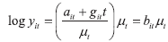 | (2) |
In this dynamic factor model μt is a common component. The coefficient bit explains how individual countries relate to the common component μt. In this paper, the focus is on fiscal convergence. Instead of looking at output per capita, we consider convergence in government debt, revenues, and expenditures. The common component μt in that case are EU institutions, integration process, and/or common policies, while bit represents a share of a common trend for each EU member state.
Coefficients bit could be empirically analyzed using relative transition curves hit which are simply the relative departure of country i from the average, or: 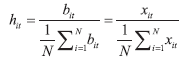 | (3) |
where xit are series on government debt, revenue, or expenditures. 2 We remove the cyclical component from the time series as suggested by Phillips and Sul ( 2009) by using the Hodrick and Prescott ( 1997) filter, but the results are not very sensitive to cyclical smoothing. Convergence is evident when hit curves for all countries approach 1.
The log t test is a more formal way for testing convergence. The test builds on relative transition curves and has the following form:  | (4) |
where 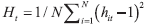 is a quadratic distance measure which goes to 0 when countries converge. t = T0 , ..., T where T0 is the first observation after we discard the initial 30% of observations, as suggested by Phillips and Sul ( 2009). Second term on LHS is a penalty function which improves test performance, and ut is an iid error. Convergence is tested with the coefficient γ. When γ is negative and statistically significant, we can conclude that countries diverge. If 0 ≤ γ < 2 we can conclude there is a conditional convergence in growth rates. For absolute convergence to hold, γ ≥ 2. 3 The critical value at 5% level significance is 1.65.
Phillips and Sul ( 2007; 2009) also developed a clustering algorithm for detecting endogenous convergence clubs based on the log t regression. If the convergence hypothesis is rejected for the full sample, club convergence can be considered. The clustering algorithm has four steps. Simplified, in the first step we sort countries in the panel, and in the second step, we form a core group of k countries, where k < N, for which the log t regression yields the highest t-statistics. 4 The remaining N – k countries form a complementary group. In the third step we add one country at the time from the complementary to the core group and for each we apply the log t test. If t > -1.65, the new country is added to the core group. The first convergence club is obtained after all countries that satisfy the condition are added. In the fourth step, we apply the log t test on the group of remaining countries which are not a part of the first convergence club. If the t-statistic is greater than -1.65, the second convergence club is identified. If not, we repeat steps (1) to (3) on the group of remaining countries to identify other possible convergence clubs.
To obtain as few clubs as possible, we run separate tests for club merging. Once initial clubs are identified, we run the log t test on them. If convergence hypothesis is not rejected for club 1 and club 2, we merge them and form a new club 1. New club 1 is then tested for merging with club 3 and so on. The advantage of this procedure is that it produces fewer convergence clubs, but the downside is that the evidence for convergence is less convincing, because the t-statistic on the γ coefficient is usually insignificant.
2.3 Unit root tests for convergence
We use different unit root tests for convergence analysis within identified clubs to check the robustness of our results. We test for convergence in government debt, revenues, and expenditures both in the full sample of EU 28 and in each identified convergence club. Following the approach of Bernard and Durlauf (1995) and Pesaran (2007) we compute a difference between country i and the average which we test for the unit root:  | (5) |
where xit represents government debt, revenues, or expenditures in country i, and x̄t is an adjusted average excluding country i under consideration. The adjusted average should prevent a bias in testing, which could be large for big countries such as Germany.
If the difference series x͂it is stationary, then there is convergence in government debt, revenues, or expenditures. Shocks to an individual country’s fiscal variables may be permanent or temporary, but all shocks to the difference series x͂it should be only temporary if country i converges to the average. Rejection of unit root is evidence of convergence. If our results are robust, rejections should be higher within identified clubs than in the full sample of EU 28.
We apply unit root tests developed by Lee and Strazicich ( 2003), and Enders and Lee ( 2012) that can control for structural breaks. Structural breaks are highly possible in government debt, revenues, and expenditures time series since they include the period of the sovereign debt crisis and the Great Recession in the EU. Ignoring structural breaks might be a serious problem that reduces the power of the test, as argued in Perron ( 1989). We also present results of a standard ADF test, which does not control for structural breaks. Intuitively, structural breaks are abrupt changes in the data such as the Great Recession. It is possible that the convergence was present both before and after the break, but the existence of the break violates our conclusions.
The Lee and Strazicich ( 2003)unit root test controls for two sharp breaks in the data. It is a Lagrange Multiplier (LM) test with the equation: 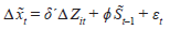 | (6) |
where S͂t is a detrended x͂t series and ϕ is a coefficient of interest. Under the null hypothesis of unit root ϕ = 0, and the rejection of unit root implies convergence.
We use the so-called break model which allows for two breaks in both level and the trend of the series using dummy variable vector Zt = [1, t, D1t, D2t, DT1t, DT2t]. Dummy variables D1t and D2t control for breaks in level and take value 1 if t ≥ TBj + 1 and 0 otherwise for breaks j = 1, 2 where TBj are break locations. On the other hand, dummy variables DT1t and DT2t control for breaks in the trend where DTjt = t – TBj for t ≥ TBj + 1 and 0 otherwise for breaks j = 1, 2. Break locations TB1 and TB2 are endogenously determined in a grid search which minimizes the t-statistics of coefficient ϕ.
Critical values for the LM test with two breaks in a level and the trend are taken from table 2 of Lee and Strazicich ( 2003). Number of lags in the equation (6) is chosen based on general to specific procedure.
We also use the Enders and Lee ( 2012) unit root test, which controls for an unknown number of smooth structural transitions approximated by a flexible Fourier function. The Fourier function has proved to accommodate smooth breaks very well, there is no need for a grid search as in Lee and Strazicich ( 2003) test, and the number of estimated parameters is relatively small, so the test does not lose power. The test equation is simple and can be estimated by OLS: 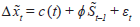 | (7) |
where again S͂t is detrended x͂t series and ϕ is a coefficient of interest. The null hypothesis of unit root assumes ϕ = 0, and again a rejection of unit root implies convergence. However, equation (7) includes a time-dependent deterministic term c(t) which is approximated by a single frequency Fourier function of the form 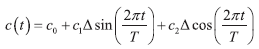 | (8) |
where c0, c1, and c2 are coefficients estimated by OLS, t is a current time period, and T is a number of observations. Note that the equation (8) nests a standard linear specification when c1 and c2 are equal to zero. We run the model with a single frequency equal to one, and with a number of lags chosen by general to specific procedure. Critical values are taken from Enders and Lee ( 2012) table 1.
2.4 Policy response function for the sustainability analysis
We analyze fiscal policy sustainability using a policy response function as suggested by Bohn (1998, 2007).5 Our model can be written as:
Equation (9) is a dynamic panel version of Bohn’s policy response function where sit is the government primary surplus in country i at time t, dit is public debt, and y͂it is the output gap. eit is the residual where eit = αit + εit , and αi are country fixed effects. The error term εit is independent, or E[εitεjk] = 0 for each i, j, t, and k where i ≠ j.
Fiscal policy is sustainable when β1 is positive, suggesting an increase in primary surplus as a response to higher public debt. Such behavior is considered sustainable and responsible, because the government tends to increase its revenue or decrease spending as a response to higher debt.
Bohn ( 1998) stressed the importance of controlling the model with the output gap.Coefficient β2 next to the output gap also tells us if the fiscal policy is pro- or countercyclical. When β2 < 0, the positive output gap decreases government surlus and fiscal policy can be considered as procyclical and vice versa (Balassone, Francese and Zotteri, 2010).
Our model includes a richer dynamic than initially proposed in Bohn ( 1998) by including a lagged primary surplus (Cassou, Shadmani and Vázquez, 2017). This specification is more appropriate because it allows for fiscal policy persistence and because of a possible feedback effect between public debt and surplus in a panel framework; accumulated government deficits (negative surpluses) are closely related to public debt.
The benchmark model is estimated by a system GMM augmented with common correlated effects (CCE) proposed by Pesaran ( 2006) to deal with cross-sectional dependence. The system GMM estimator proposed by Arellano and Bover ( 1995), and Blundell and Bond ( 1998) is often used for dynamic panel estimation, and we use their two-step procedure with robust standard errors where fixed effects are removed by first differencing. 6
Our panel consists of European Union countries which are somewhat homogenous in terms of common institutions and policies, and therefore a cross-sectional dependence can be an important issue affecting our results. 7 To deal with the issue of cross-sectional dependence, we augment the system GMM estimator by adding cross-sectional means of all variables as instruments in the model from the equation (9). Common correlated effects procedure is proposed by Pesaran ( 2006) for a group of OLS estimators. However, we use this principle to augment system GMM estimator. Pesaran ( 2006) showed that adding CCE has satisfactory small sample properties for relatively small N and T even in heterogeneous models. We call this model system GMM-CCE model.
We confirm the robustness of the benchmark model by estimating a dynamic panel model with fixed effects (FE) using robust errors. Our data set is a balanced panel with a reasonably large T = 62 and therefore the FE estimator should not be biased. We refer to this model simply as the FE model.
3 Fiscal convergence and sustainability
3.1 Convergence clubs
We do not find any evidence to support the absolute convergence of government debt, revenues, and expenditures in the EU using relative transition curves and log t test. The relative transition curves in figure 1 show lack of convergence, because they do not approach 1 in the observed period. By contrast, curves are scattered equally at the beginning and the end of the sample.
Figure 1Relative transition paths DISPLAY Figure
This is further supported by a more formal log t test presented in table 1. Table 1 shows γ coefficient from the log t regression applied to government debt (1a), revenues (1b), and expenditures (1c) data. Again, γ < 0 implies divergence, 0 ≤ γ < 2 is evidence of conditional convergence, and γ ≥ 2 implies absolute convergence in levels. Table 1 shows that γ coefficient is significantly negative (marked with an asterisk) when log t test is applied to all EU countries, which rejects absolute convergence of government debt, revenues, and expenditures. Kočenda, Kutan and Yigit ( 2008) also find fiscal divergence in a form of pronounced level of heterogeneity in public debt and deficit among EU member states.
We also find that the Great Recession and sovereign debt crisis further increased fiscal divergence in the EU. In figure 2 we show results of estimated rolling window γ coefficient for government debt, revenues, and expenditures. We estimate the log t regression with a centered rolling window of 20 quarters (five years) together with 95% confidence intervals. For all three variables, estimates are significantly negative throughout the observed period, which further confirms the result of fiscal divergence. An interesting finding is that the estimated γ further decreases from 2008 in the case of government revenues and expenditures and from 2011 in the case of government debt. Therefore, it could be argued that the Great Recession and sovereign debt crisis pushed the EU further away from fiscal convergence.
Table 1log t convergence test results and convergence clubs classification DISPLAY Table
However, we find strong evidence of club convergence. Convergence clubs are implicitly included in discussions about the EU core and periphery as well as in the idea of two-speed recovery in Europe popularized by Blanchard ( 2010). We use the clustering algorithm of Phillips and Sul ( 2007, 2009) to determine convergence clubs endogenously. Results are presented in table 1 under Club classification section. Countries that form convergence clubs are shown in figure 3.
Table 1a presents results for government debt. We find two convergence clubs, one containing 19 and the other 9 countries. The γ coefficient is statistically zero in the first, and positive, but less than 2 in the second club, which indicates conditional convergence of clubs. Similarly, for government revenues, three convergence clubs emerged and club sizes are 19, 5, and 3 (table 1b). Ireland and Romania form a divergence group, since they do not converge to any club. For government expenditures, club classification finds five clubs in total, plus Ireland as a divergent group. However, clubs 3 and 4 can be merged together according to log t test, so the final classification shows four convergence clubs plus Ireland (table 1c). Club sizes are 5, 11, 9, and 2 for Clubs 1, 2, 3, and 4 respectively. In each case 0 ≤ γ < 2 indicating conditional convergence.
Figure 2Rolling window estimation of log t regression DISPLAY Figure
Identified clubs are heterogeneous in a sense that countries within a club do not share common geographical, political, or development similarities. In figure 3 we show countries that form different clubs. The first row of figure 3 shows clubs from 1 to 4 and divergent groups. The first column indicates fiscal variables: government debt, revenues, and expenditures. Convergence clubs are in squares, while divergent groups are in circles. For example, government debt Club 1 includes Croatia, Cyprus, Estonia, Hungary, Lithuania, Romania, Slovakia, and Slovenia, which are new member states, mostly small countries, and most of them experienced the transition from centrally planned to market economy. However, Austria, Belgium, Finland, France, Greece, Ireland, Italy, Portugal, Spain, Sweden, and the UK are also members of the same club (government debt Club 1). Similar diversity can be found within other clubs.
Figure 3Convergence clubs DISPLAY Figure
We find a substantial degree of homogeneity in government debt, revenues, and expenditures clubs. For example, government debt Club 1 and government revenues Club 1 share 12 of 19 countries (figure 3). All eleven countries in government expenditures Club 2 are also in government debt Club 1. There is a major overlap between government debt Club 2 and government expenditures Club 3. Other similarities can also be observed in figure 3. Therefore, clubs are heterogeneous within countries, but homogenous in fiscal variables.
Endogenously identified clubs indeed show evidence of convergence, but this is not the case for ad-hoc exogenous clubs. First, we group countries into EU-15 and EU-13 and apply the log t regression to government debt, revenues, and expenditures data. The results reject convergence in all cases except for government debt in EU-13, where the γ coefficient is statistically equal to zero (0.042 with a t-statistic of 1.34). Next, we group countries into EU core and periphery 8 and use the log t test. Convergence is strongly rejected in both groups for all three fiscal variables. It seems that countries converge to some criteria other than simply geographical, political, or development similarities, or indeed multiple similarities. 9 These results could be compared with Kočenda, Kutan and Yigit ( 2008) who analyze fiscal convergence in the ten EU countries that joined EU in 2004. They do not find a systematic difference among all EU countries, EU core, and EU periphery when analyzing fiscal convergence. Delgado ( 2006) uses cluster analysis to group EU countries thus avoiding ad-hoc exogenous clubs, but the paper does not tackle the issue of fiscal club convergence.
The log t regression improves upon the standard β-convergence tests, but results are compatible with such tests. In figure 4 we show a simple scatter plot of government debt level and a growth rate, which is a version of an unconditional β-convergence test. For government debt Clubs 1 and 2, we estimate the equation of the form log (dTi/d1i) = α + β d1i + εi, where the dependent variable is the debt growth rate between the last and the first period, and the independent variable is a debt level in the first period. Club 1 is depicted with black circles, and Club 2 with grey pluses. As shown in the figure 4, regression lines for each club are negatively sloped indicating convergence within clubs according to the standard β-convergence test.
Figure 4β-convergence in clubs DISPLAY Figure
3.2 Unit root tests of fiscal convergence
Table 2 presents results of fiscal convergence using unit root tests for the sample of 28 EU countries and within clubs identified by the clustering algorithm. For the government debt data, we analyze convergence to the average for the full sample of the EU 28, then for the 19 countries of convergence club 1, and then for the 9 countries of club 2 (table 2a). A similar analysis is done for government revenues and expenditure in table 2b and 2c, respectively. For each club, we compute a separate adjusted average. Unit root rejection rates at 10% significance level are presented for ADF, Lee and Strazicich (2003), and Enders and Lee (2012) test. Rejection of the unit root hypothesis is considered evidence of convergence.
Table 2Club convergence using unit root tests DISPLAY Table
We find neither absolute nor club convergence in government debt data because the difference of government debt against the average is stationary for just a few countries. For the full sample of EU 28, unit root rejection rates are only 3.5% in the case of ADF and the Lee and Strazicich test, and 7% for the Enders and Lee test. Rejection rates within two clubs are not much different, thus not supporting club convergence of government debt.
In the case of government revenues and expenditures, we do not find evidence of absolute convergence, but club convergence is supported. Almost half of countries in the EU 28 sample converge to the average. ADF test has low power in the presence of structural breaks, but the unit root is rejected in 35% to 40% of countries for both series. The Enders and Lee test has more power and rejects the unit root in 46% of countries. Finally, the Lee and Strazicich test with sharp structural breaks shows the biggest rejection rates of 78% and 85%. For both government revenues and expenditures, rejection rates within clubs are higher than in the full sample of EU 28, indicating stronger convergence within clubs. This is especially true for Lee and Strazicich ( 2003) test where rejection rates are mostly over 90% within clubs indicating strong club convergence. Enders and Lee ( 2012) test has rejection rates within clubs well over 50%, except in government revenues club 2 and government expenditures club 1. ADF test gives somewhat mixed results but does not reject the club convergence hypothesis. This confirms that convergence clubs using the Phillips and Sul ( 2007; 2009) clustering algorithm are robust, except for government debt. As a comparison, De Bandt and Mongelli ( 2000) use cointegration techniques to analyze fiscal convergence in the Eurozone. Their findings support fiscal convergence in the Eurozone over the 1970-1998 period. Unit root tests which allow for nonlinearities have recently been a more popular way of analyzing convergence (see Raguž Krištić, Rogić Dumančić and Arčabić ( 2018) and references therein).
3.3 Fiscal (un)sustainability
Next, we analyze if fiscal policy is sustainable in the European Union and within convergence clubs found in the previous section. In this respect, we use the policy response function from equation (9) which relates primary government surplus with public debt and the output gap. If surplus increases as a response to an increase in public debt, fiscal policy is considered sustainable, as discussed in the methodology section.
We analyze fiscal sustainability using seven different models (subsamples). Model 1 is the benchmark model, which includes 28 EU countries. Models 2 and 3 include subsamples of countries from government debt convergence clubs identified in the previous section. The first club consists of 19, and the second of 9 countries. 10 Next, we consider fiscal policy sustainability within exogenous clubs of EU-15 and EU-13 countries with Models 4 and 5. Finally, Models 6 and 7 use subsamples with government debt ≥ 90% (Model 6) and debt < 9% of GDP (Model 7). This subsample analysis is motivated by the influential paper of Reinhart and Rogoff ( 2010) who argue that a public debt higher than 90% of GDP depresses economic growth. Maastricht criteria also require government debt below 60% of GDP. However, EU countries fought with the Great Recession and the sovereign debt crisis, which substantially increased the level of public debt in some countries. Our data show that 15 out of 28 EU countries had a government debt higher than 60% of GDP in 2017:Q2. Therefore, such subsample analysis is interesting from both an academic and a policy perspective. The 90% level of public debt can be considered as arbitrary, especially since Arčabić et al. ( 2018) show there is no single level of public debt associated with the decrease of GDP growth. However, in this paper, we are only interested in fiscal sustainability.
Fiscal policy is found to be unsustainable in the EU. We present the results of system GMM-CCE and FE estimators in tables 3 and 4, respectively. Different models are numbered in the first row of each table, and independent variables are in the first column. In table 3, the estimated coefficient β1 next to the government debt is negative or insignificant. In other words, the government does not increase primary surplus as a response of higher government debt, and fiscal policy is not sustainable. We find weak evidence of fiscal sustainability for the EU-13 group countries and for the subsample with debt ≥ 90%. For these two models (Models 5 and 6), point estimates are positive with both system GMM-CCE and FE estimator. However, coefficients are insignificant for system GMM-CCE estimator, and point estimates are small in magnitude in both cases (tables 3 and 4).
Fiscal policy is countercyclical in the EU and in all subsamples considered. Balassone, Francese and Zotteri ( 2010), and Cassou, Shadmani and Vázquez ( 2017) use β2 coefficient next to the output gap to analyze cyclicality of fiscal policy. As presented in tables 3 and 4, the coefficient next to output gap is positive and statistically significant in all models. 11 Positive output gaps are related to an increase in primary surplus, which can be interpreted as a countercyclical fiscal policy. This indicates that fiscal policy in the European Union tries to smooth business cycles.
Fiscal policy is fairly persistent because the coefficient ρ next to the lagged surplus is positive, statistically significant, and roughly 0.5.
Table 3Results of fiscal sustainability analysis using system GMM-CCE model DISPLAY Table
Table 4Results of fiscal sustainability analysis using FE model DISPLAY Table
4 Conclusion
The Great Recession and the sovereign debt crisis in the Eurozone have shaken fiscal policies in the EU. Many European countries have breached public debt and deficit goals set by the Stability and Growth Pact. Therefore, the issue of fiscal policy convergence and sustainability is very important for the EU.
This paper analyzes fiscal policy convergence and tests for fiscal sustainability in 28 EU countries using data on government debt, revenues, and expenditures. We show absolute divergence in fiscal policies, which was further increased by the Great Recession and the sovereign debt crisis. However, we find strong evidence of club convergence. Club convergence is important to consider because the EU does not have a single fiscal policy and member state policies are heterogeneous. In general, convergence clubs are implicitly included in discussions on the EU core and periphery, and in the two-speed recovery idea which argues that different groups (or clubs) of European countries are characterized by faster and slower recoveries from the recession. We find two government debt convergence clubs, three government revenue clubs, and four government expenditure clubs. Endogenously identified clubs do not have simple geographical, political, or development similarities. They are heterogeneous within countries, but homogenous between fiscal variables. Exogenous grouping of EU countries into EU-15 and EU-13 or into EU core and periphery does not show evidence of fiscal convergence. Convergence clubs are related to multiple equilibriums within the EU, which makes a single fiscal policy difficult to achieve. More precise fiscal rules could be considered by policymakers together with corrective measures such as the Excessive Deficit Procedure. Fiscal rules instead of discretionary decision making might be a step toward similar fiscal policies and fiscal convergence in the EU.
Fiscal policy in the EU is found to be unsustainable, but countercyclical. We use a policy response function for the sustainability analysis where primary surplus is a function of government debt and the output gap. We show that surplus does not respond to an increase in government debt, which cannot be interpreted as sustainable. However, primary government surplus increases in expansions and decreases in recession, thus being countercyclical and aimed at smoothing business cycles. In this respect, the fiscal goals for public debt and deficit set by the Stability and Growth Pact may not be enough to ensure fiscal sustainability. More precise fiscal rules together with corrective measures would be helpful for both fiscal sustainability and convergence.
Appendix
DATA CONSTRUCTION AND SOURCES
For the convergence analysis, we use data on general government debt, revenues, and expenditures. Variables are in millions of euro, current prices. We divide all by nominal GDP to express fiscal variables in real terms and in a percent of GDP. The main data source is Eurostat and the International Financial Statistics database from the International Monetary Fund. All data span the period from 2000:q1 to 2017:q2, but some data have been reconstructed. For Germany, Estonia, Ireland, and Luxemburg we interpolate annual data for 2000 and 2001 since quarterly data start from 2002:q1. For Austria, we interpolate annual data for 2000 since quarterly data start from 2001:q1. For Croatia, we reconstruct monthly dana on central government expenditure and revenue based on the old methodology. The data are provided by Croatian National Bank (CNB) and we use central government data as a proxy for the general government. Nominal GDP is taken from the Eurostat database except for Croatia, Malta, and Poland for which we take the data from IFS. Public debt data are entirely taken from the Eurostat database. Public debt is usually expressed as a percent of GDP on annual bases. Therefore, public debt is divided by a sum of GDP in a current and previous three quarters, or dt = 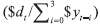 x 100, where dt is public debt in a percent of GDP, $ dt, and $ yt are nominal debt and GDP in millions of euro. We use this approach for the sustainability analysis when the sample starts in 2002:q1. For the convergence analysis where the sample starts in 2000:q1, we divide public debt only by current quarter GDP to maximize number of observations, or dt = ($ dt /$ yt) × 100. For the sustainability analysis, we also use primary surplus and real GDP data from Eurostat. All the data span the period from 2002:q1 to 2017:q2 (balanced panel). Below we plot time series of government revenues and expenditures (figure A1), and primary surplus and government debt (figure A2) in a percent of GDP. Table A1 contains basic descriptive statistics.
Figure A1Government revenues and expenditures as a percent of GDP DISPLAY Figure
Figure A2Primary surplus and government debt as a percent of GDP DISPLAY Figure
Table A1Descriptive statistics DISPLAY Table
Data construction and sources
Funding
This work has been supported in part by Croatian Science Foundation under the project 6785.
Notes
* The author would like to thank Junsoo Lee, Robert J. Sonora, Hrvoje Šimović, Josip Tica, Tomislav Globan, Kyoung Tae Kim, Ozana Nadoveza Jelić, Irena Raguž Krištić, Yu You, and two anonymous referees for helpful comments on the paper.
1 1997-2003 period is considered.
2 For each variable we run a separate test.
3 Phillips and Sul (2007; 2009) provide more technical details of the test. For empirical analysis we use a set of procedures described in Du (2017).
4 To form a group, the t-statistic for parameter γ from log t regression must be t > -1.65.
5 Bohn (2005; 2007) criticize fiscal sustainability analysis based on unit root and cointegration techniques popularized by Trehan and Walsh (1988) and Hamilton and Flavin (1986). He argues that such techniques are not capable of rejecting sustainability hypothesis because the relevant debt variables are necessary stationary after a finite number of differencing and thus in compliance with the intertemporal budget constraint (IBC).
6 We use first differencing instead of forward orthogonal deviaton (FOD) because our data set is a balanced panel. Refer to Arellano and Bover (1995) and Blundell and Bond (1998) for complete technical details.
7 Indeed, when we apply Pesaran (2015) test for weak cross-sectional dependence to the model, the null hypothesis of cross-sectional independence can be easily rejected.
8 EU core countries are Austria, Belgium, Denmark, Finland, France, Germany, Luxembourg, Netherlands, Sweden, and UK. Other 18 countries form EU periphery.
9 Analysis of factors and criteria to which countries converge is beyond the scope of this paper.
10 We consider government debt convergence clubs only, but clubs are fairly homogeneous between fiscal variables, as discussed. In addition, some government revenues and expenditures convergence clubs include only a few countries, which is impractical for panel data analysis.
11 Only Model 6 in table 4 has a positive, but insignificant output gap.
* The author would like to thank Junsoo Lee, Robert J. Sonora, Hrvoje Šimović, Josip Tica, Tomislav Globan, Kyoung Tae Kim, Ozana Nadoveza Jelić, Irena Raguž Krištić, Yu You, and two anonymous referees for helpful comments on the paper.
1 1997-2003 period is considered.
2 For each variable we run a separate test.
3 Phillips and Sul ( 2007; 2009) provide more technical details of the test. For empirical analysis we use a set of procedures described in Du ( 2017).
4 To form a group, the t-statistic for parameter γ from log t regression must be t > -1.65.
5 Bohn ( 2005; 2007) criticize fiscal sustainability analysis based on unit root and cointegration techniques popularized by Trehan and Walsh ( 1988) and Hamilton and Flavin ( 1986). He argues that such techniques are not capable of rejecting sustainability hypothesis because the relevant debt variables are necessary stationary after a finite number of differencing and thus in compliance with the intertemporal budget constraint (IBC).
6 We use first differencing instead of forward orthogonal deviaton (FOD) because our data set is a balanced panel. Refer to Arellano and Bover ( 1995) and Blundell and Bond ( 1998) for complete technical details.
7 Indeed, when we apply Pesaran ( 2015) test for weak cross-sectional dependence to the model, the null hypothesis of cross-sectional independence can be easily rejected.
8 EU core countries are Austria, Belgium, Denmark, Finland, France, Germany, Luxembourg, Netherlands, Sweden, and UK. Other 18 countries form EU periphery.
9 Analysis of factors and criteria to which countries converge is beyond the scope of this paper.
10 We consider government debt convergence clubs only, but clubs are fairly homogeneous between fiscal variables, as discussed. In addition, some government revenues and expenditures convergence clubs include only a few countries, which is impractical for panel data analysis.
11 Only Model 6 in table 4 has a positive, but insignificant output gap.
Disclosure statement
No potential conflict of interest was reported by the author.
References
Arčabić, V. [et al.], 2018. Public Debt and Economic Growth Conundrum: Nonlinearity and Inter-temporal Relationship. Studies in nonlinear dynamics and econometrics, 22(1), pp. 1-20 [ CrossRef]
Arellano, M. and Bover, O., 1995. Another look at the instrumental variable estimation of error-components models. Journal of econometrics, 68 (1), pp. 29-51 [ CrossRef]
Balassone, F., Francese, M. and Zotteri, S., 2010. Cyclical asymmetry in fiscal variables in the EU. Empirica, 37(4), pp. 381-402 [ CrossRef]
Bernard, A. B. and Durlauf, S. N., 1995. Convergence in international output. Journal of applied econometrics, 10(2), pp. 97-108 [ CrossRef]
Bernard, A. B. and Durlauf, S. N., 1996. Interpreting tests of the convergence hypothesis. Journal of econometrics, 71(1-2), pp. 161-173 [ CrossRef]
Blundell, R. and Bond, S., 1998. Initial conditions and moment restrictions in dynamic panel data models. Journal of econometrics, 87(1), pp. 115-143 [ CrossRef]
Bohn, H., 1998. The behavior of US public debt and deficits. The Quarterly Journal of economics, 113(3), pp. 949-963 [ CrossRef]
Bohn, H., 2005. The Sustainability of Fiscal Policy in the United States. CESifo Group Munich. Working paper, No. 1446.
Bohn, H., 2007. Are stationarity and cointegration restrictions really necessary for the intertemporal budget constraint? Journal of monetary economics, 54(7), pp. 1837-1847 [ CrossRef]
Cassou, S. P., Shadmani, H. and Vázquez, J., 2017. Fiscal policy asymmetries and the sustainability of US government debt revisited. Empirical economics, 53(3), pp. 1193-1215 [ CrossRef]
Collignon, S., 2012. Fiscal policy rules and the sustainability of public debt in Europe. International economic review, 53(2), pp. 539-567 [ CrossRef]
Delgado, F., 2006. Are the tax mix and the fiscal pressure converging in the European Union? Instituto de Estudios Fiscales Working paper, No. 11-06.
Deskar-Škrbić, M. and Šimović, H., 2017. Effectiveness of fiscal spending in Croatia, Slovenia, and Serbia: The role of trade openness and public debt level. Post-communist economies, 29(3), pp. 336-358 [ CrossRef]
Enders, W. and Lee, J., 2012. A unit root test using a Fourier series to approximate smooth breaks. Oxford bulletin of economics and statistics, 74(4), pp. 574-599 [ CrossRef]
Hamilton, J. D. and Flavin, M. A., 1986. On the Limitations of Government Borrowing: A Framework for Empirical Testing. American economic review, 76(4), pp. 808-819.
Hodrick, R. J. and Prescott, E. C., 1997. Postwar US business cycles: an empirical investigation. Journal of money, credit, and banking, 29(1), pp. 1-16 [ CrossRef]
Kočenda, E., Kutan, A. M. and Yigit, T. M., 2008. Fiscal convergence in the European Union. The North American Journal of Economics and Finance, 19(3), pp. 319-330 [ CrossRef]
Lee, J. and Strazicich, M. C., 2003. Minimum Lagrange multiplier unit root test with two structural breaks. Review of economics and statistics, 85(4), pp. 1082-1089 [ CrossRef]
Perron, P., 1989. The great crash, the oil price shock, and the unit root hypothesis. Econometrica, 57(6), pp. 1361-1401 [ CrossRef]
Pesaran, M. H., 2006. Estimation and inference in large heterogeneous panels with a multifactor error structure. Econometrica, 74(4), pp. 967-1012 [ CrossRef]
Pesaran, M. H., 2007. A pair-wise approach to testing for output and growth convergence. Journal of econometrics, 138(1), pp. 312-355 [ CrossRef]
Pesaran, M. H., 2015. Testing weak cross-sectional dependence in large panels. Econometric reviews, 34(6-10), pp. 1089-1117 [ CrossRef]
Phillips, P. C. and Sul, D., 2007. Transition modeling and econometric convergence tests. Econometrica, 75(6), pp. 1771-1855 [ CrossRef]
Phillips, P. C. and Sul, D., 2009. Economic transition and growth. Journal of applied econometrics, 24(7), pp. 1153-1185 [ CrossRef]
Raguž Krištić, I., Rogić Dumančić, L. and Arčabić, V., 2018. Persistence and stochastic convergence of euro area unemployment rates. Economic Modelling [ CrossRef]
Reinhart, C. M. and Rogoff, K. S., 2010. Growth in a Time of Debt. American economic review, 100(2), pp. 573-578 [ CrossRef]
Trehan, B. and Walsh, C. E., 1988. Common trends, the government's budget constraint, and revenue smoothing. Journal of economic dynamics and control, 12(2-3), pp. 425-444 [ CrossRef]
|


