3175
Views
381
Downloads |
Introducing a composite indicator of cyclical systemic risk in Croatia: possibilities and limitations
Tihana Škrinjarić* 
Article | Year: 2023 | Pages: 1 - 39 | Volume: 47 | Issue: 1 Received: June 1, 2022 | Accepted: November 3, 2022 | Published online: March 6, 2023
|

FULL ARTICLE
FIGURES & DATA
REFERENCES
CROSSMARK POLICY
METRICS
LICENCING
PDF
Source: Author’s adjustment based on OECD (2012).
|
Full name
|
Risk category covered
|
Unit measure
|
|
New bank loans to households
|
Credit developments
|
Q sum of monthly new loans
|
|
New bank loans to nonfinancial corporations
|
|
Property prices
|
Potential overvaluation of property prices
|
Year-on-year change
|
|
Household debt and gross disposable income
ratio
|
Private sector debt burden
|
Year-on-year growth rate
|
|
Nonfinancial corporations debt and gross
operating surplus ratio
|
|
Spread between rate on new loans to households
and 3M PRIBOR (multiplied with -1)
|
Potential mispricing of risk
|
% annually
|
|
Spread between rate on new loans to
nonfinancial corporations and 3M PRIBOR (multiplied with -1)
|
|
PX 50 stock index
|
Three-month average
|
|
Adjusted current account deficit and GDP ratio
(multiplied with -1)
|
External imbalances
|
% annually
|
Note: All variables in the table in the described form indicate that the greater the value, the greater the risk accumulation is. Source: Plašil et al. (2015).
|
Risk category
|
Variables
|
Transformation
|
|
Cyclogram
|
Cyclogram+
|
|
Lending market
|
Credit-to-GDP gap HH
Credit growth HH
Credit growth NFC
|
Credit-to-GDP gap HH
Credit-to-GDP gap NFC
Credit growth HH
Credit growth NFC
|
HP gaps
Differences
|
|
Risk appetite
|
NPL values
Default rates of NFC
|
NPL values HH
NPL values NFC
Default rates of NFC
Interest rate margin HH
Interest rate margin NFC
|
Everything in levels
|
|
Indebtedness
|
Indebtedness of HH
Indebtedness of NFC
|
Both in HP gaps and levels
|
|
Property market
|
Residential property price
Price to income ratio
|
Residential property price
Residential property price in main city
Price to income ratio
Price to rent ratio
Flat to house price ratio
|
Growth rate and levels
|
|
Macroeconomy
|
ESIŽUnemployment rate
Output gap
|
ESI
Unemployment rate
Output gap
Revenue gap
Current account deficit to GDP ratio
|
HP gaps and levels
|
Note: The gap denotes the HP gap, NPL denotes nonperforming loans, HH and NFC are households and nonfinancial corporations, y-o-y is the year-on-year change or growth rate, ESI is the economic sentiment indicator. All variables in the table in the described form indicate that the greater the value, the greater the risk accumulation is. Source: Rychtarik (2014, 2018).
|
Indicator
|
Transformation
|
Method of data aggregation
|
Data selection criteria
|
Advantages
|
Shortfalls
|
|
FCI
|
Order statistics
|
Nonlinear function (like portfolio variance)
|
Financial cycle theory, previous literature, without
empirical evaluation of the variable characteristics before the crisis.
|
Takes correlation into consideration, graphical
representation, no problems with statistical filters regarding data
transformation, robustness due to scaling variables.
|
Lack of objective data selection criteria, variable
selection affects the dynamics of the indicator, harder to communicate, hart
to evaluate the results
|
|
Cyclogram
|
Max min or based on percentiles of distribution
|
Average, weighted average
|
Previous experience with variable dynamics tracking.
|
Graphical representation, no problems with
statistical filters regarding data transformation, easy aggregation and
interpretation
|
|
d-SRI
|
Normalization, standardization or max min
|
Early warning models of signaling crisis.
|
Data selection criteria, simple aggregation and
interpretation, robust9
|
Correlations not observed, biased results for one
country analysis
|
|
PCA
|
Normalization, standardization
|
Weighted average based on loadings on the first
principal component
|
Any of the previous three main approaches
|
Simple aggregation
|
Assumptions of PCA analysis, changing correlations,
bad predictive power of the first principal component.
|
|
Geometric average
|
Normalization, standardization
|
Geometric average formula
|
Hard to interpret results in economic way,
correlations not observed, depends on the main method of aggregation,
negative values in data.
|
|
RMS
|
Normalization, standardization
|
Root mean square formula
|
Hard to interpret results in economic way,
correlations not observed, depends on the main method of aggregation,
negative values in data, lack of risk accumulation in one category is
substituted with high risk in other.
|
|
OI
|
Binary variable depending on EWM results
|
Average or weighted average
|
If based on d-SRI approach, advantages as there
|
Hard to interpret results in economic way,
correlations not observed, depends on the main method of aggregation,
negative values in data.
|
|
Abbreviation
|
Transformation
|
Variable
|
Risk category
|
FCI variant
|
|
ΔICSN
|
Yearly growth rate
|
House price index
|
Potential overvaluation of property prices
|
(1)
|
|
A. 2ΔICSN
|
Annualized two-year growth rate
|
(2)
|
|
ΔKK
|
Yearly growth rate
|
Bank loans to households
|
Credit dynamics
|
(1)
|
|
A. 2ΔKK
|
Annualized two-year growth rate
|
(2)
|
|
ΔKNFP
|
Yearly growth rate
|
Bank loans to nonfinancial corporations
|
(1)
|
|
A. 2ΔKNFP
|
Annualized two-year growth rate
|
(2)
|
|
Δ(LR)
|
Yearly change
|
Leverage ratio
(multiplied with -1)
|
Strength of bank balance sheets
|
(1)
|
|
A. 2Δ(LR)
|
Annualized two-year change
|
(2)
|
|
Δ(LTD)
|
Yearly change
|
Credit to deposit ratio
|
(1)
|
|
A. 2Δ(LTD)
|
Annualized two-year change
|
(2)
|
|
Δ(K/Y)
|
Yearly growth rate
|
Debt (households) to disposable income ratio
|
Private sector debt burden
|
(1)
|
|
A. 2Δ(K/Y)
|
Annualized two-year growth rate
|
(2)
|
|
Δ(NFP/BOV)
|
Yearly growth rate
|
Debt (nonfinancial corporations) to gross operating
surplus ratio
|
(1)
|
|
A. 2 Δ(NFP/BOV)
|
Annualized two-year growth rate
|
(2)
|
|
ΔCROBEX
|
Yearly growth rate
|
CROBEX, stock market index
|
Mispricing of risk
|
(1)
|
|
A. 2 ΔCROBEX
|
Annualized two-year growth rate
|
(2)
|
|
Δ margin K
|
Yearly change
|
Household credits interest rate margin (difference
between average new credits interest rate to households and 3 month EURIBOR
interest rate)
(multiplied with -1)
|
(1)
|
|
A. 2 Δ margin K
|
Annualized two-year change
|
(2)
|
|
Δ margin NFP
|
Yearly change
|
Nonfinancial corporations credits interest rate
margin (difference between average new credits interest rate to nonfinancial
corporations and 3 month EURIBOR interest rate)
(multiplied with -1)
|
(1)
|
|
A. 2 Δ margin NFP
|
Annualized two-year change
|
(2)
|
|
ΔRN
|
Yearly change
|
Current account to GDP ratio (multiplied with -1)
|
External imbalances
|
(1)
|
|
A. 2 ΔRN
|
Annualized two-year change
|
(2)
|
Source: CNB, author’s calculation.
|
Variant (1)
|
Variant (2)
|
|
Combination of variables that are transformed to
annualized two-year changes or growth rates, and HP gaps, 125.000 value of
the smoothing parameterr14.
|
Variant with GDP and unemployment dynamics.
|
Source: CNB, author’s calculation.
|
Risk
categories
|
Indicator
description
|
|
Credit dynamics measures
|
HP gap for the broad
definition of credit to households, smoothing parameter of 125,000
|
|
HP gap for the broad
definition of credit to non-financial corporations, smoothing parameter of
125,000
|
|
HP gap for the ratio of
narrow definition of credit and the sum of GDP of the current quarter and the
preceding three quarters, smoothing parameter of 125,000
|
|
Measures of credit
institution financing risk
|
Annualized two-year change
in the negative ratio between credit institutions’ equity and assets
|
|
Annualized two-year change
in the negative ratio between private sector deposits and credit
|
|
Measures of potential real
estate price overvaluation
|
Annualized two-year growth
rate in the residential real-estate price index
|
|
Annualized two-year growth
rate in the residential real-estate price-to-disposable income ratio
|
|
Annualized two-year growth
rate in the volume index of construction works
|
|
Measures of private sector
debt burden
|
HP gap for the ratio
between corporate debt and gross operating surplus, smoothing parameter of
125,000
|
|
HP gap for the ratio
between household debt and disposable income, smoothing parameter of 125,000
|
|
HP gap of debt service
measures – households, smoothing parameter of 125,000
|
|
HP gap of debt service
measures – corporations, smoothing parameter of 125,000
|
|
Measures of external
imbalances
|
Annualized two-year change
in the negative share of net exports of goods and services in GDP
|
|
Annualized two-year change
in the negative share of current account balance in GDP
|
|
Measures of potential
mispricing of risk
|
Annualized two-year growth
rate in CROBEX
|
|
Annualized two-year change
in the negative interest margin on new loans to households relative to the
3-month EURIBOR
|
|
Annualized two-year change
in the negative interest margin on new corporate loans relative to the
3-month EURIBOR
|
Source: CNB, author’s calculation.
|
Variant
|
Description
|
|
Variant (1)
|
Variables from table 6, normalization via median and
standard deviation of each variable.
|
|
Variant (2)
|
Variables from table 6, normalization via max-min
approach of each variable.
|
Source: CNB, author’s calculation.
|
Indicator
|
error T1
|
error T2
|
Sum
|
Weight (%)
|
|
HP gap,
household credit
|
0,08
|
0,08
|
0,16
|
8,84
|
|
HP gap,
nonfinancial corporations credit
|
0,08
|
0,21
|
0,29
|
4,47
|
|
HP gap,
narrow definition of credit
|
0,00
|
0,41
|
0,41
|
2,84
|
|
2y change,
equity to assets ratio
|
0,50
|
0,00
|
0,50
|
2,15
|
|
2y change,
deposit to credit ratio
|
0,00
|
0,09
|
0,09
|
15,82
|
|
2y growth
rate, house price index
|
0,00
|
0,13
|
0,13
|
11,09
|
|
2y growth
rate, house price to income ratio
|
0,00
|
0,09
|
0,09
|
17,14
|
|
2y growth
rate, volume index of construction works
|
0,00
|
0,00
|
0,00
|
8,00
|
|
HP gap,
ratio debt to gross operating surplus
|
0,00
|
0,22
|
0,22
|
6,10
|
|
HP gap,
ratio debt to disposable income
|
0,00
|
0,49
|
0,49
|
2,24
|
|
HP gap,
debt service ratio, households
|
0,00
|
0,49
|
0,49
|
2,24
|
|
HP gap,
debt service ratio, nonfinancial corporations
|
0,00
|
0,33
|
0,33
|
3,73
|
|
2y growth
rate, net exports to GDP ratio
|
0,00
|
0,61
|
0,61
|
1,57
|
|
2y growth
rate, current account to GDP ratio
|
0,08
|
0,45
|
0,53
|
1,95
|
|
2y growth
rate, CROBEX
|
0,00
|
0,00
|
0,00
|
8,00
|
|
2y change,
interest margin, households
|
0,33
|
0,16
|
0,49
|
2,22
|
|
2y change,
interest margin, nonfinancial corporations
|
0,25
|
0,19
|
0,44
|
2,60
|
Note: Abbreviations refer to variables from table 6, the following the sequence from first to last one as in the mentioned table. Source: CNB, author's calculation.
Source: CNB, author’s calculation.
Source: CNB, author’s calculation.
Source: CNB, author’s calculation.
Source: CNB, author’s calculation.
|
|
|
Abstract
This research deals with several approaches to constructing a composite indicator of cyclical systemic risk accumulation with a specific focus on Croatia. Such indicators are important in macroprudential policymaking, in order to track the position of the economy in the financial cycle. Moreover, the countercyclical capital buffer (CCyB) depends on the timely and accurate estimation of cyclical risk accumulation. The credit gap as defined in the BCBS (Basel Committee on Banking Supervision) and the ESRB (European Systemic Risk Board) guidance and recommendation has shown many flaws in practice. Thus, there is a need for improvement of the methodology. That is why this paper deals with the advantages and shortfalls of existing composite indicators of cyclical systemic risks and the possibilities of introducing them in Croatia. This research contributes to a critical overview of the methodological approaches, with suggestions for their improvement, focusing particularly on the specifics of Croatian data.
Keywords: cyclical risk; macroprudential policy; composite indicator; systemic risk
JEL: C14, C32, E32, 344
1 Introduction
One of the tasks of macroprudential policy is to track the cyclical systemic risks and estimate the economy’s position within the financial cycle (Constâncio et al.,  2019). The reasoning is that such information is used to assess the macroprudential policy stance based on the information on existing risks, the resilience of the financial system, and the policy itself. If the policy could dampen the peaks and troughs of the financial cycle itself, it would result in positive societal benefits. As one of the main tasks of macroprudential policy is to reduce the cyclical nature of the financial cycle and reduce systemic risks when they accumulate, there is a need for continuous monitoring of indicators that help to discover the phase of the cycle in which a specific financial system is located. The Basel credit gap is considered a stepping stone in financial cycle evaluation. It is estimated as the difference between the credit-to-GDP ratio and its long-term trend calculated via the HP filter (Hodrick and Prescott, 1997). Also, macroprudential authorities use the Basel credit gap as a basis for the calibration of the CCyB (Countercyclical capital buffer)1 to increase the resilience of the financial system. 2019). The reasoning is that such information is used to assess the macroprudential policy stance based on the information on existing risks, the resilience of the financial system, and the policy itself. If the policy could dampen the peaks and troughs of the financial cycle itself, it would result in positive societal benefits. As one of the main tasks of macroprudential policy is to reduce the cyclical nature of the financial cycle and reduce systemic risks when they accumulate, there is a need for continuous monitoring of indicators that help to discover the phase of the cycle in which a specific financial system is located. The Basel credit gap is considered a stepping stone in financial cycle evaluation. It is estimated as the difference between the credit-to-GDP ratio and its long-term trend calculated via the HP filter (Hodrick and Prescott, 1997). Also, macroprudential authorities use the Basel credit gap as a basis for the calibration of the CCyB (Countercyclical capital buffer)1 to increase the resilience of the financial system.
The HP filter is the most commonly used way to estimate the Basel gap, in practice and in the literature (see BIS, 2011; ESRB, 2014; Drehmann and Tsatsaronis, 2014; Dell’Ariccia et al., 2012; Rünstler and Vlekke, 2016; Wezel, 2019, Škrinjarić and Bukovšak, 2022). However, there are many problems with using this indicator for measuring the accumulation of cyclical systemic risk. Some of the well-known problems include the following. The gap calculated via the HP filter (Hodrick and Prescott, 1997) is biased because of the prolonged period of excessive credit growth before the GFC (Lang et al., 2019; Galán, 2019). This means that it will take longer to close the credit gap and positive rates of CCyB will be activated only when it is too late. The HP filter is characterized by the end-point problem (Canova, 1998; Pedersen, 2001; Edge and Meisenzahl, 2011) due to greater weights given to the latest observations in the optimization function. This can affect the decision-making process concerning the values of the CCyB rate, making it unreliable in real time. Next, the credit gap is often non-stable and/or nonstationary (Kauko, 2012a; Geršl and Seidler, 2012; Rychtarik, 2014; Castro, Estrada and Martínez, 2016). Consequently, unreliable unwanted CCyB rate variations could be problematic. Furthermore, the HP filter also has problems regarding the smoothing parameter that determines the length of the financial cycle itself, as ESRB ( 2014) proposes the value of 400,000. This implicitly assumes that all economies have an equal length of the financial cycle (30 years), a fact that is not true in practice (see Rünstler and Vlekke, 2016; Valinskytė and Rupeika, 2015; Wezel, 2019) 2.
Also, much recent research has found other variables to be good signalling indicators of the financial cycle and future turn of the cycle. The meta-analyses of Castro, Estrada and Martínez ( 2016), BIS ( 2017), and Tölö, Laakkonen and Kalatie ( 2018) offer a good overview of empirical work done so far. As can be seen there, more than 90 variables were found to be helpful in modelling and predicting the financial cycle. The authors have found that observing information not only about credit developments but asset prices, housing dynamics, external imbalances, private sector debt burden, mispricing of risks, the strength of bank balance sheets, etc. facilitate the modelling process of the financial cycle itself, and consequently, the decision-making process of important macroprudential issues. However, when dealing with many data at once, policymakers are synthesizing the information into one single measure, a composite indicator of cyclical systemic risk. For example, in a recent study, Arbatli-Saxegaard and Muneer ( 2020) overview current central bank practices in the CCyB rate decision-making process. It shows that European countries included in the research use 6 to 35 different individual variables as indicators within the analysis of the cyclical risk build-up. Other newer applications of composite indicators are found in Plašil et al. ( 2015) and Plašil, Seidler and Hlaváč ( 2016) for the Czech National Bank; Lang et al. ( 2019) for EU countries and Rychtárik ( 2014, 2018) in Slovakia. Based on developments in different risk categories, the common factor of all these approaches is that all the information is summarized in composite indicators that facilitate the risk monitoring process. Composite indicators are, thus, useful to determine the economy’s position within the financial cycle on the one hand and to provide detailed information about the dynamics of individual indicators that enter the composite indicator itself, on the other hand. Moreover, research proves that using such composite indicators helps mitigate systemic financial crises and their adverse effects on output (see Laeven and Valencia, 2012; Lo Duca et al., 2017).
That is why this paper gives a critical overview of the existing composite indicators regarding their motivation, methodology, advantages, and shortfalls. Based on these findings, comments about possible improvements can be applied in general, as well as regarding Croatian data. The empirical part of the paper will evaluate the possibilities of constructing an indicator for Croatia. The macroprudential policymaker can observe changes in the total cyclical systemic risk accumulation by obtaining such results in a composite indicator. In more detail, the sources form different risk categories. Furthermore, such an indicator offers insights into the financial conditions of the economy, providing signals of cyclical risk build-up. As financial systems are complex, the cyclical risk build-up can be observed better through a composite indicator. When the composite indicator is defined in practice, it is instrumental in giving information about the aggregate cyclical risk behaviour. It also provides information about the dynamics within sub-categories of the indicator itself, which should be monitored according to Comelli and Ogawa ( 2021). This is some of the reasoning on why such an indicator is better in practice than the Basel credit gap. Taking everything into consideration, the whole process is, of course, challenging. That is why many central banks use heat maps to consider cyclical risks. Although the main conclusions are obtained via some aggregation, a sole indicator is harder to obtain. This is corroborated by Arbatli-Saxegaard and Melle Johansen ( 2017), where the authors argue that a heat map can capture the complex set of information and factors about the financial cycle. Aikman et al. ( 2015), in their review of the IMF, Offices of Financial Research, and Bank of England approach to financial cycle monitoring, conclude that all three institutions employ a significant number of indicators, with two of them using heat maps as visualization tools (alongside spider charts) to summarize all of the information better.
Focusing on Croatian data could be interesting for international readers for the following reasons. Croatia has had one of the most proactive macroprudential policies ever since the early 2000s, actively attempting to manage credit growth alongside capital inflows (see Kraft and Galac, 2011). This is especially true for the pre-GFC period, as Croatia was at the forefront of the creation of a timely countercyclical macroprudential policy (Vujčić and Dumičić, 2016). Thus, some specific happenings in the economy and financial sector, alongside the macroprudential activity of the Croatian National Bank (CNB), could be beneficial for other countries or those whose authorities are becoming more active.
A composite indicator can be used in the next step to calibrate the CCyB values concerning the evaluation of the position of the financial cycle. Thus, managing an active CCyB rate can help mitigate systemic risk crises over time, which have resulted in significant losses in the past (see Laeven and Valencia, 2012; Lo Duca et al., 2017). Finally, the purpose of constructing a composite indicator of cyclical systemic risk in this research is threefold. It could be used to determine the phase of the financial cycle, some components could be used as early warning indicators, as they are based on such methodology, and it could be a good tool for communication with the public, as changes in its components can be interpreted more efficiently than by the individual tracking of dozens of indicators.
2 General information about composite indicators and variable selection
2.1 About composite indicators in general
Cyclical composite indicators are discussed in handbooks such as the one by the EU and UN (2017). They list the main characteristics of such indicators, such as objectivity, freedom from bias, methodological soundness, clarity, transparency, interpretability, consistency, comparability, and readability. This is hard to achieve in practice, as the selection process of variables of interest has some bias due to the analysis of specific issues as well as occasional interpretability issues, depending on the approach of constructing the composite indicator itself. Other necessary and desirable properties are described in OECD (2012), which states that variables included in the composite indicator should have economic relevancy, the highest data frequency possible, without many data revisions, series breaks or publication lags. This is almost impossible to achieve in practice due to the nature of the data being observed and monitored for the analysis of cyclical behaviour, dealing with quarterly data that is usually published with a lag of several months in some cases, etc.
Figure 1 depicts the basic steps that need to be followed to construct a reliable indicator. The procedure seems straightforward at first, but many issues arise at each step. Step one includes the variable selection process, which depends on theory and/or empirical research, to correctly determine relevant indicators that represent the phenomenon. Due to the individual variables being expressed in different measurement units, the second step includes proper data preparation (normalization or standardization) to be comparable. Moreover, if the idea is to measure specific dynamics, e.g., seasonality in data is an excess, it should be properly removed. The third step compares all potential candidate variables from steps one and two based on the primary goal of the indicator. For example, if the main idea is to construct a leading indicator, then forecasting methods are utilized to compare the variables in their forecasting properties. Finally, when the individual variables are ranked concerning their performance in step three, the last step aggregates all information into one composite indicator. Here, the main question concerns the distribution of weights across the individual indicators. Of course, in practice, the process is not so straightforward, and some of the steps will repeat.
Figure 1Composite indicator construction steps DISPLAY Figure
2.2 Variable selection for the composite indicators
This section describes general ideas and explanations about several categories of risk measures that need to enter a composite cyclical risk indicator. The reasons for the importance of these variables for measuring cyclical risk movements are also explained. As the ESRB ( 2014) Recommendation has six categories of variables that indicate the build-up of system-wide risk associated with periods of excessive credit growth, a good composite indicator should include variables that follow within these categories. They include measures of potential overvaluation of property prices, credit developments, external imbalances, the strength of bank balance sheets, private sector debt burden, and potential mispricing of risk.
The category of potential overvaluation of property prices consists of variables that are most common in good early prediction of financial crises. Borio ( 2012), Jordá, Schularick and Taylor ( 2012), and Behn et al. ( 2013), among others, find that overvaluation of property prices in combination with excessive credit growth is the best early warning signalling variable. The movements of loans in the economy and real estate prices are highly correlated. This is because real estate purchase is usually financed by lending. Moreover, such loans make up a large part of banks’ balance sheets, making them vulnerable to large changes in real estate prices (Tölö, Laakkonen and Kalatie, 2018). The wealth effect is one of the incentives for higher real estate demand (Bakker, 2015), which creates price pressures in the upward phase of the financial cycle. This further stimulates credit expansion due to the increased value of the collateral (Bernanke and Gerlter, 1995; Kiyotaki and Moore, 1997). According to some research, property price movements have even preceded credit dynamics in some countries (see Grinderslev et al., 2017). Property price movements are sources of risk for households, corporations, and credit institutions. High property prices burden the private sector that finances house purchasing via bank loans. This can reduce the rest of private consumption. In addition, credit institutions hold real estate as collateral, which affects the value of balance sheets and price changes.
Credit dynamics is probably most commonly monitored in practice and investigated in empirical research. This is due to lending being the core business of credit institutions and thus affecting financial stability and cyclical risk accumulation. Alongside the property price dynamics, credit dynamics and developments have been proposed as the best predictors of crises in previous research (see Borio and Lowe, 2002; Borio and Drehmann, 2009; or Aldasoro, Borio and Drehmann, 2018). In periods of economic growth, optimism rises, and a reduced perception of risk characterizes economic agents. Expectations about future revenues are high, the private sector is more prone to taking loans, and credit institutions are more inclined to giving them to riskier clients (Plašil, Seidler and Hlaváč, 2016). Changing risk tolerance is assumed concerning the state of the economy, wealth, and balance sheets. These concepts are not new, as changeable risk aversion and tolerance were found in Minsky ( 1975, 1982, 1986). Here, the financial instability hypothesis states that after the turbulent period of the financial cycle is over, the economy is on a new path towards equilibrium and the recovery phase is in financial tranquillity. Policymakers and financial regulators are easing their regulatory standards, credit spreads are falling, and lenders are starting to approve loans they otherwise would not. At the same time, borrowers are showing speculative behaviour, and lending is increasing until a financial crisis materializes, with rising interest rates and declining lending. Then, the recovery phase follows, and the cycle continues. This relates to Borio and Zhu ( 2011), where the changing risk tolerance is related to monetary policy and its effects on credit institution behaviour. It explains the risk-taking channel as the effects of interest rate change on risk perceptions, which is reflected in the riskiness of the bank portfolio.
There is evidence that loans granted during a period of economic expansion have a greater default rate than those made in periods of slow credit growth (see Jimenéz, Salas and Saurina, 2006). Credit cycle studies are mostly focused on private sector credit growth and overheating, such as Babecký et al. ( 2014), Schularick and Taylor ( 2012), Borio and Drehmann ( 2009), Giese et al. ( 2014). Furthermore, as Jordà, Schularick and Taylor ( 2013, 2017) find, deeper recessions follow credit-intense booms and, empirically, financial factors and credit play an essential role in business cycle dynamics. The private sector debt burden has been considered both theoretically and empirically (see Rinaldi and Sanchiz-Arellano, 2006). If the debt burden is too high, this reduces financial stability. Accumulation of debt burden in the private sector in the short run affects consumption and GDP growth. In the long run, it spills over onto the whole financial system (Lombardi, Mohatny and Shim, 2017). This is the reason why a part of the literature is focused on monitoring variables within this group of measures, where it examines the debt burden or debt servicing ratios (see Giese et al., 2014; Detken et al., 2014; Drehmann and Juselius, 2012, 2014). As Plašil, Seidler and Hlaváč ( 2016) explain, accelerated debt-to-income ratio growth can indicate that the private sector overestimates its future possibility of debt repayment. This means that there is a decrease in solvency as a consequence of the worsening of the financial situation.
Measures of external imbalances are related to credit growth in an economy outstripping growth in GDP and domestic savings (Tölö, Laakkonen and Kalatie, 2018). The current account deficit is interpreted as investment in the economy greater than the sum of private and public savings (Plašil, Seidler and Hlaváč, 2016). This can lead to future problems with repayment of loans obtained from abroad (Giese et al., 2014). In Laeven and Valencia’s ( 2008) study, in total 39 out of 41 economies had a current account deficit in the years that preceded financial crises in the past. Other relevant variables that were found to be informative of future crises were net exports, capital account dynamics, terms of trade, and gross external debt, as found in a meta-analysis by Tölö, Laakkonen and Kalatie ( 2018). Interested readers can refer to Kaminsky, Lizondo and Reinhart ( 1998), which gives a review of currency crises as they are related to external imbalances.
Banking sector vulnerability should also be visible in banks’ balance sheets. However, there are some problems regarding variables within this group of measures. Tölö, Laakkonen and Kalatie ( 2018) found that these variables are rarely used as there is a publication lag of such measures, based on balance sheets and financial reports. Research finds significant and non-significant future crisis prediction results based on such variables. For example, Detken et al. ( 2014) found that the study’s capital-to-asset ratio (the leverage ratio) had poor predictive power. On the other hand, Laina, Nyholm and Sarlin ( 2015) and Kamin and DeMarco ( 2012) found that a greater leverage ratio had future stabilizing effects on the financial system. In that way, the capital of a credit institution should be able to serve as a measure of the loss-absorbing capacities when the private sector stops repaying the loans. The greater the capital, the smaller the probability of future deleveraging during the financial downturn. Moreover, the economy-wide debt and leverage dynamics directly relate to such bank credit and leverage dynamics. With some economies, such as the US, it was important in non-bank credit as well.
This group also includes the ratio of (negative value) deposits and credit to the private sector, providing information about financing from stable sources, not depending on issuing securities or financing by borrowing.
Measures of potential mispricing of risk include distorted risk perceptions of the private sector and the bank sector. Distorted risk perception during some phases of the financial cycle can contribute to the accumulation of systemic risk. That is why this group of measures includes financing conditions variables, which measure the risk perception of credit institutions. Bordalo, Gennaioli and Shleifer ( 2018), López-Salido, Stein and Zakrajšek ( 2017), and Gross ( 2022) show that credit spreads fall during boom times. Furthermore, such falling spreads actually reflect rising risk, due to structurally falling volatility, disguising/dominating rising risk from growing indebtedness/leverage. Thus, this group of measures includes the interest premium regarding the private sector over a referent interest rate (such as the national interest rate or Euribor). Moreover, there are different economic accelerator types, defined and depicted in detail in Gross ( 2022). They include the collateral one (Bernanke, 1999, collateral value is procyclical and amplifies mispricing during upswings), mispricing (Jiménez, Salas and Saurina, 2006, regarding lending standards), herding behaviour (Kirman, 1992), and others. Other measures of risk mispricing are stock prices and their dynamics, as they can complete the total picture (Plašil et al., 2015). To summarize, Pfeifer and Hodula ( 2018) explain that credit institutions have greater estimation errors during the expansion phase of the financial cycle on the future non-repayments of given loans. If the share of nonperforming loans in total loans is very small at the peak of the financial cycle, credit institutions are realizing profits that are cyclically over-estimated. Thus, a bank prudence indicator is developed in the mentioned study by Pfeifer and Hodula ( 2018). It represents another measure of potential mispricing of risk, and it depends on such explanations.
Finally, as some approaches include some macroeconomic variables as additional information in the modelling process, here we examine the dynamics of business cycles. Rychtarik ( 2014) offers some reasoning on why macroeconomic variables should be tracked and explains that financial institutions could fuel macroeconomic imbalances, i.e., there could be spillovers of risk accumulation onto the real sector as well. Detken et al. ( 2014) add that macroeconomic imbalances and conditions affect the ability to repay loans (e.g., an increase in unemployment increases credit risk). Moreover, monetary indicators could also reflect problems: changes in money supply could affect asset prices (Adalid and Detken, 2007). Another example is foreign debt, which could reflect differences between information that the foreign lender and domestic creditors have (Kauko, 2012b).
3 Review of composite indicators for financial cycles
3.1 Financial cycle indicator
3.1.1 General description of FCI
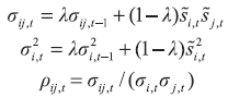
The financial cycle indicator (FCI) developed by Plašil et al. (2015) estimates the economy’s position within the financial cycle. The authors select the main variables that enter FCI with respect to the previous theoretical literature (such as Borio, 2012; or Borio and Zhu, 2011). In these works the financial cycle is observed via changing risk assessment by different economic agents. In the upswing of the cycle, the FCI indicator is interpreted as the risk accumulation within the financial system with respect to changed risk perceptions of different economic agents. Greater optimism in one sector should contribute to a greater FCI value. Moreover, if several sectors have similar risk perceptions, this should also be reflected in greater FCI values, i.e. correlation among the dynamics of risk perceptions matters within this approach. Formal construction of this indicator is based on Holló, Kremer and Lo Duca (2012). w = (w1 , w2 , ..., wM) is the vector of weights i, i ∈ {1, 2, ..., M}, values of transformed variables are given in vector st = (st,1, st,2, ..., st,M) for every period t, and FCIt indicator in period t is a nonlinear function constructed as:
| FCIt = (w ⊙ st)' ∙ Ct ∙ (w ⊙ st) | (1) |
 | (2) |
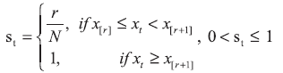
 are the values of each series reduced by the median value. Values si,t are obtained from original data in x = (x1 , x2 , … , xN), ordered from the smallest to the greatest value: (x[1], x[2], ... , x[N]), x[1] ≤ x[2] ≤ ... ≤ x[N], where [r] is the rank of value x[r] . And finally, values st are obtained from the empirical cumulative function distribution as follows: are the values of each series reduced by the median value. Values si,t are obtained from original data in x = (x1 , x2 , … , xN), ordered from the smallest to the greatest value: (x[1], x[2], ... , x[N]), x[1] ≤ x[2] ≤ ... ≤ x[N], where [r] is the rank of value x[r] . And finally, values st are obtained from the empirical cumulative function distribution as follows:
 | (3) |
Table 1Variables used in Plašil et al. (2015) for FCI indicator DISPLAY Table
3.1.2 Comments about the fci indicator
The original paper does not fully describe the selection of variables for FCI. Although the selected variables make sense as they cover basic risk categories, there is no explanation of the chosen unit measures, the appropriateness of the selected variables, or their comparison to other relevant ones within each risk category5. There are some issues with the method of covariance estimations. EWMA assumes that the dynamics of covariances and variances are the same for all series (the same smoothing parameter). Unfortunately, there is no universal answer about how to choose this parameter. An ideal way to determine this value would be to minimize some of the forecasting measures (such as root mean squared error, see Bollen, 2014) in which the value of FCI is compared to a true realized volatility. Next, the data used in constructing the FCI indicator is on a quarterly frequency, and the variables are more sluggish than not. Therefore, it is advisable to use a greater value in such an analysis. Also, the greater the value of this parameter, the smaller the standard error of the variance estimator. In terms of costs and benefits for capturing the systemic risk, there are not many differences between larger or smaller lambda values besides smoothing out the final value of the composite indicator.
Moreover, the EWMA approach is more parsimonious than more complicated approaches, such as the DCC (dynamic conditional correlation). However, such an approach needs many more available data to obtain reliable estimations, something which is currently not available for Croatian data. Finally, another problem is how to determine the weights of each variable in the composite indicator. Practice often employs equal weights within a sub-category so that individual variables do not affect the outcome in a great manner. Another approach is found in Hájek, Frait and Plašil ( 2017). In this paper, the authors forecast future nonperforming loans (NPL) dynamics as a risk materialization variable using the FCI indicator. A final suggestion on how the weights can be determined is to estimate the EWM for every variable included in the indicator and give greater weights to those that had better predictive performances in crises.
3.2 Cyclogram and cyclogram+
3.2.1 General description of the cyclogram
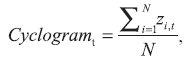
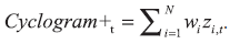
The cyclogram was developed in Slovakia in Rychtarik (2014, 2018). It is based on a linear aggregation of several risk measures categories. The basic approach here is to define core variables that determine the cycle. Afterward, the information is completed with supplementary variables (such as unemployment dynamics, consumer sentiment, etc.). There are two versions of this indicator: the cyclogram and the cyclogram+ (greater number of variables). The variable selection process is not detailed in the original research, as authors describe that the selection was made by the usual monitoring process of cyclical risks, especially based on the dynamics of the variables before GFC. The value of the cyclogram in every quarter t is calculated as the simple average value of the transformed variables zi,t as follows:
 | (4) |
 | (5) |
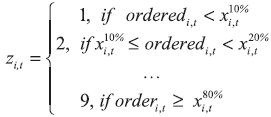 | (6) |
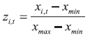 | (7) |
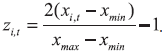 Table 2 lists the variables included in the cyclogram. However, there is a problematic part in macroeconomic variables. Since they follow a business cycle, their dynamics lag. For example, when a downturn of the GFC happened, the changes in unemployment lagged compared to other variables, which captured the pre-crisis accumulation of risk. In addition, some variables are monitored in their levels and some in form of change (via change or statistical gaps). This makes the decision somewhat subjective and hard to communicate. Table 2 lists the variables included in the cyclogram. However, there is a problematic part in macroeconomic variables. Since they follow a business cycle, their dynamics lag. For example, when a downturn of the GFC happened, the changes in unemployment lagged compared to other variables, which captured the pre-crisis accumulation of risk. In addition, some variables are monitored in their levels and some in form of change (via change or statistical gaps). This makes the decision somewhat subjective and hard to communicate. Table 2List of variables used in the cyclogram (and +) DISPLAY Table
3.2.2 Comments about the cyclogram
The basic idea of the cyclogram is not much different from that of the FCI indicator, but correlations are not included in the analysis. Variable weights are given based on equal weights to all variables in the first version of the indicator, which was redefined into equal weights across groups of variables. The monitoring of other relevant variables, macroeconomic, for instance, is important for obtaining a bigger picture. However, the idea of a composite cyclical systemic risk is to calibrate CCyB values on time. Thus, the use of unemployment rates and NPLs is inappropriate due to their lagging behaviour compared to the turning points of the business or financial cycles. This is prominent in Croatian data as well. Whereas NPLs are used in the FCI approach to forecasting them via the leading values of FCI, here the cyclogram consists of NPLs to determine the general value of the risk accumulation. This could be detrimental for CCyB calibration, especially when taking it into consideration that the CCyB value determined in a quarter of some year is put into practice one year later.
3.3 Domestic systemic risk indicator (D-SRI)
3.3.1 General description of D-SRI
Domestic systemic risk indicator (d-SRI henceforward) was developed in Lang et al. (2019) as an ECB publication. Since then, this indicator has regularly appeared in macroprudential reports, at least at the EU or EA level. This indicator is based on the results from early warning models (EWM) of signalling financial crises on a panel of countries across several financial crises over the decades. This makes the d-SRI primarily an empirical approach to constructing the composite indicator itself. Lang et al. (2019) observe many different variables and their transformations. The value of d-SRI for a country in every quarter is calculated as the average value of transformed variables that were the best in the EWM approach:
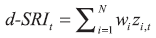 | (8) |
 | (9) |
| ujt = Γj + γ1ujt-1 + εujt | (10) |
3.3.2 Comments about D-SRI
The variable selection process here is objective and clear, due to EWM being a basis for variable comparison. Although future crises will not necessarily have the same causes, a starting point is needed. Thus, it is possible to use the EWM procedure to select a core group of variables that should be important when tracking risk accumulation. On the other hand, like others in this study, this approach relies on historical data and the observation of specific dynamics before and during crises that will not necessarily be repeated in the future. Therefore, such modelling should consider this issue and be flexible and adjustable. As the original paper utilizes panel data, the normalization process can be performed as noted in the previous sub-section. However, when dealing with non-normal data, other transformations are better. This could be the rank or the max-min. In addition, when dealing with one country or crisis in the sample, such as the Croatian case, it is possible to give equal weights over every risk category, to minimize the estimation bias. In that way, if the policymaker decides to change the structure of a risk category by including new variables or excluding existing ones, the weighting scheme allows the final indicator value not to be greatly affected (as it would be by, e.g., removing a variable from the sample).
3.4 Other popular methods of aggregation of data
3.4.1 Principal components analysis
Principal components analysis (PCA) is used for correlated variables, where the original dataset is converted into a new set of uncorrelated principal components. PCA can be useful to reduce the analysis’s dimensionality when the original dataset has many variables. One recent application to determine the financial cycle is found in Karamisheva et al. (2019). However, PCA analysis rests upon a number of assumptions, such as the linear relationship between the variables, the first two moments of the variable distributions being enough to describe them, etc., see Jackson (1991).
3.4.2 Overheating index
The overheating index (OI) is suggested in Chen and Svirydzenka (2021). The authors rely on the EWM model to obtain the signalling properties of every variable that was a potential candidate to enter the composite indicator. But, compared to the d-SRI, the basis on which the OI is constructed is the values of the variables that exceed a certain threshold value. A binary variable Ii is defined as equal to 0 value if the original value does not exceed a threshold and 1 otherwise. Now, the OI indicator is calculated as:
 | (11) |
3.4.3 Aikmann et al. (2015) approach
Aikmann et al. (2015) examine several approaches to aggregating data into one indicator. The following is the main formula for aggregating data:
 | (12) |
3.5 Comparison of the selected approaches
Based on the previous overview of the selected approaches, we can compare their advantages, shortfalls, and some possibilities for Croatian data application. In general, all composite indicators are good at summarizing the information within each risk category into one number. It would be more difficult to track the dynamics of individual indicators in parallel, especially when the CCyB values need to be calibrated. However, the differences are as follows.
Table 3Summary of the three main approaches for composite indicator construction DISPLAY Table
Variable selection in some approaches is arbitrary. For example, the FCI study does not define how to transform variables. Other approaches, such as the d-SRI and OI, are based on the EWM approach of determining which variables and transformations were the best in signalling previous crises, which reduces subjectivity 10. Such data selection approaches are better for country comparisons, as the variables are set. Moreover, the results can be comparable across the financial cycle and across a set of countries. By focusing more on individual indicators, it is possible to state that the FCI indicator has the advantage of including the correlation structure in its construction. If more variables tell the same story, we are more convinced that the risks are accumulating. However, this complicates the interpretation of the results. If the value of the indicator increases, we cannot be sure if this is due to an increase in the value of an individual variable, or due to the correlation 11 dynamics. The cyclogram in the original paper had the advantage of not using statistical filters and their problems (as described in the introduction).
Next, if we look at the data aggregation possibilities afterward, the approach of Aikmann et al. ( 2015) could have problems with negative data values. This makes the interpretability of the results harder. Policymakers have to consider communication with the public. A simple average is more worth considering. The OI index is a good starting point from which to extend the d-SRI indicator to obtain reliable results when one has more data and crises in the sample. As the OI approach is based on referent thresholds from the EWM model, it is problematic in the case of Croatia, due to the specific movements of the variables before the only crisis in the sample. This means that some referent values will not be exceeded in the future. The indicator would not show us the need to impose a positive value of CCyB, but it will be needed in reality. The PCA is a simple approach to analysis due to the focus on the first principal component results. However, there is one more problem in this approach, alongside those mentioned. When we use short time series, such as Croatian data, it is hard to test the validity of the assumptions. A summary of the three main approaches is given in table 3, alongside the comments on the rest of the approaches to aggregating the data.
4 Empirical analysis
4.1 Brief data description
Quarterly series of the following data were collected for the empirical part of the study. All six risk accumulation categories are covered, as described in the second section. The starting point of a time series is 4Q 1999, with some variation due to lack of data. One such is the property price dynamics, which starts in 1Q 2002. The end of the sample is 3Q 2021. Nominal and real values of specific variables were obtained, broad and narrow definitions (credit), one and two-year differences, growth rates, one-sided HP gaps for 1.600, 25.600, 85.000, 125.000, and 400.000 values of smoothing parameters in the filtering process, dividing the data into that regarding households versus nonfinancial corporations, etc. For example, in the credit dynamics category, we look at both broad and narrow credits, their ratio to GDP, and all mentioned transformations. In the external imbalances category, we look at gross and net external debt, their ratios to GDP, terms of trade, current account to GDP ratio, net exports to GDP ratio, all their transformations, etc. Accordingly, the study compares more than 260 different variables in total12.
4.2 FCI estimation results
All data were transformed into two-year differences or growth rates to obtain better smoothness of individual variables and the composite indicator itself. The original FCI paper uses the current account to GDP ratio in levels due to different dynamics compared to Croatian data. In the original form, the current account is non-stationary. Thus, we use differences instead of level values. Table 4 gives a summary of the two approaches. The first FCI variant includes yearly changes and growth rates (as in the original paper). The second variant uses annualized twoyear changes and growth rates. All variables are given equal weights.
Figure 2 depicts the two variants of the FCI indicator in panels A. and B. Firstly, the FCI indicator increases significantly before the GFC due to the credit dynamics, house price increases, and changes in bank balance sheet strengths. After the indicator reached its maximum value at the beginning of 2007, there was a great fall in FCI value. As of 2017, a mild recovery is found until the end of the sample. The average correlation contribution is plotted alongside the dynamics of individual variables, as it is usually difficult to track all pairs of correlations in the model. Some variables do not have a significant positive correlation over time, meaning that the average correlation will contribute to the reduction of the total FCI indicator. Thus, the correlation contribution is plotted as negative values. For example, after 2018, the FCI indicator’s value is much lower than in the period before the GFC due to variables having a lower correlation overall.
Figure 2 shows that it is relatively easy to follow the dynamics of individual variables that enter the composite indicator alongside the FCI value. However, due to the data transformation, it is harder to interpret the low-risk phase of the financial cycle. Therefore, it would be more straightforward to look at data with both positive and negative values, as this would be easier to comprehend. Moreover, as mentioned previously, the final value of the composite indicator depends not only on the dynamics of the individual variables but the correlation structure, not shown in figure 2. Finally, some variables had a later starting point. This, in turn, resulted in a relatively short period of the FCI indicator (beginning in 2004), as the correlation matrix estimation requires equal length of all series.
Table 4Summary of two FCI variants DISPLAY Table Figure 2Selected FCI indicators and their dynamics DISPLAY Figure
4.3 Cyclogram estimation results
The cyclogram is the second indicator in focus. There are some problems here with including non-performing loans13, as this variable has a lagging value compared to others that capture changes in the cycle with the preceding dynamics. Something similar holds for the macroeconomic: GDP and unemployment. The problem is that these variables also have lagging dynamics compared to changes in other variables that capture risk accumulation over time. That is why we observe two variants of the cyclogram in table 5. All risk categories will have equal weights.
Table 5Cyclogram variants for Croatian case DISPLAY Table Figure 3Cyclogram variants from table 5 DISPLAY Figure
The results are shown in figure 3. Data transformation is done as in formula (6), meaning that all of the values are positive again, as were for the FCI case. The average value of risks is captured in the cyclogram value. However, it now shows dynamics that are harder to explain compared to the FCI values. Here, it seems that the economy is almost on the same level of risk as it was before the GFC. This is due to obtaining an average value of all positive values, without the negative correlation reduction. We know that the dynamics in the last couple of years is not as dramatic as it was at the beginning of the sample 15.
4.4 d-SRI estimation results
Based on the AUROC values from the EWM approach16, we chose those indicators that are best in their respective risk category. Table 6 summarizes the properties of variables selected for every risk category.
Although the estimation process results are somewhat biased due to there being only one crisis in the sample, the variables chosen in table 6 overlap with related literature in the vast majority. However, it is advisable to track other relevant variables in parallel. Figure 4 depicts two variants of the d-SRI indicator based on data from table 6: panel A is the version with the median and standard deviation transformation procedure, whereas panel B is based on the max-min transformation of data. We include the latter transformation as normality tests rejected the null hypothesis for most variables in the study. Lang et al. ( 2019) do not recommend normalization and standardization if the data is not normally distributed. We see a specific increase in all risk categories in the early 2000s and before the GFC. The Croatian domestic developments perhaps happened to correlate with broader worldwide trends pre-GFC, in the US and Europe, even for structural reasons (trade and financial connectedness). However, it is worth mentioning that Croatia did not cause the pre-GFC vulnerabilities in the US or the GFC outbreak. The risks have been accumulating again in the last couple of quarters, specifically in the categories of property price overvaluation, increasing credit dynamics and private sector debt burden. On panel B, we opt to use max-min transformation, due to data non-normality.
Table 6Best indicators chosen for d-SRI calculation DISPLAY Table Figure 4d-SRI indicator variants DISPLAY Figure
4.5 Other selected approaches estimation results
4.5.1 PCA approach of weights selection
Since this approach requires standardization, we observe two variants of PCA aggregation, shown in table 7 and figure 5. The resulting dynamics is a similar to another and the dynamics in figure 4. The reasoning is that PCA results have almost equal variable weights. A problem here, which is found besides the theoretical problems and assumptions, is that the two resulting PCA indicators describe 50.16% and 48.68% of the total variance. So, it seems more reasonable to use equal weights without additional analysis.
Table 7Variants of PCA aggregation DISPLAY Table Figure 5Composite indicators based on PCA aggregation DISPLAY Figure
4.5.2 Overheating index weights selection and aggregation
When dealing with short time series, the thresholds are estimated within EWM result in values that cannot be realistically assumed for the future. This is due to specific values before the GFC in the case of Croatian data. However, for the sake of completeness, we obtain those threshold values for the best indicators from table 6 and follow the original paper to calculate the weights shown in table 8. The greatest values are given to the house price to income ratio, deposits to credit ratio, house price index, and household credits. As an alternative, we calculate the OI indicator based on equal weights for all variables as well. Figure 6 depicts both indicators, with some additional dynamics in figure 7 regarding the structure of the indicator, due to greater volatility in some individual variables, the overall OI indicator in both variants in figure 6 in some specific quarters. All risk categories contributed to the total OI value in the pre-GFC period. This corresponds to the previous indicators. In the last couple of years, the main contributors to risk accumulation were balance sheet strength, property price overvaluation and external imbalances. Two additional OI indicators in figure 8 are shown as well. The median value of each indicator is used as a threshold value, to obtain stable results.
Table 8Weights assignment based on errors type 1 and 2 DISPLAY Table Figure 6OI indicator, based on weights in table 8, and equal weights DISPLAY Figure Figure 7Structure of OI indicator, number of variables exceeding referent value, equal weights DISPLAY Figure Figure 8OI indicator, weights from table 8 and equal weights, median value for thresholds DISPLAY Figure
4.5.3 The Aikmann et al. (2015) approach
As a final approach to data aggregation, we look at the variants in Aikmann et al. (2015): the geometric mean calculation and the RMS (root mean square) approach. Variables are used from the d-SRI case, and the transformation is based on FCI approach. Figure 9 shows the geometric mean (panel A) and the RMS approach (panel B). The nature of calculating these indicators, especially multiplying the variables in the geometric mean setting, makes it is difficult to interpret the structure of panel A in figure 9. More intuition is given in panel B, in the RMS approach. But, squaring all variables and the final calculation of the root mean of the final value introduces nonlinearity in the procedure. Nevertheless, both indicators capture the dynamics in a way similar to that of the previous approaches, which is good. Thus, these approaches could be used as auxiliary indicators. Figure 9Geometric mean and RMS approaches of aggregating data DISPLAY Figure
4.6 Discussion based on the results
In this section we focus more on what we noticed in dealing with real data. To use any of these indicators or approaches in practice, we need to keep in mind that the variable selection needs to be as objective as possible, as this will ensure the validity of results to use in future tracking of cyclical risks. We need to include some subjectivity since some variable transformations have similar dynamics but one transformation is more stable than the other. For example, two-year growth rates in some cases had similar dynamics to the HP gaps for the smoothing parameter of 1,600. If we assume that a variable follows a business cycle dynamic and length in Croatia, the two-year growth rate tells almost the same story as the HP gap. The way in which to transform data in order to calculate the final indicator value, in terms of normalization, standardization, order statistics, max-min approach, was also a complex task. The more complicated the data transformation procedure is, the harder it is to communicate the results and decisions based on the indicator to the public. When dealing with real data, it is frequently found that the assumption of normality is often not satisfied. This was, of course, the case with Croatian data as well. Hence, the max-min approach to data transformation could be the best solution at the present time.
Data aggregation proves to be important in relation to the communication issue as well. Nevertheless, due to the combination of data transformations, and the way of aggregating it, some indicators resulted in dynamics that are hard to interpret in economic terms. For example, the cyclogram results were such that the risk values of the composite indicator were almost on the level that obtained before the GFC, which is not a realistic result (see footnote 18). In addition, the dynamics of most of the variables in the last couple of years are still somewhat subdued. Some have a rising tendency, but the increase is not as near as recorded at the beginning of the sample. Data transformations need to be somewhat refined.
In general, the most promising results are obtained using the best features of several approaches: the d-SRI approach relying on the EWM to determine the best crisis predictors, the max-min transformation of data from the cyclogram, and general visualization of the results, such as the FCI or the OI index. Here, the variables are chosen based on the EWM approach to signalling the previous crisis. There is some bias in such results, but that is why the threshold values are not used in determining the final value of the composite indicator. Instead, just those variables that were the best predictors should be considered and monitored more closely. Other additional approaches of data aggregation observed in the last empirical part showed that they could provide some additional robustness checking of the results. On the other hand, nonlinear approaches to data aggregation could potentially be hard to carry out in practice 17. Finally, the d-SRI approach is most likely to be used the most in practice, as the ECB reports utilize this indicator in country comparisons, alongside this variant being used in macroprudential stance estimation (see Krygier and Vasi, 2021; Duarte, Feliciano and De Lorenzo Buratta, 2022; or Galán and Rodríguez-Moreno, 2020).
Finally, this study focused on some approaches to cyclical risk tracking, namely the statistical filtering approach of calculating credit gaps, the composite indicator approach as the main focus, and the early warning model approach within the composite indicator. Other possible approaches that are found in practice are the semi-structural models (e.g., unobserved components model with economic and finance fundaments); multivariate models (e.g., vector error correction, where the equilibrium level of credit dynamics is estimated); other early warning approaches, such as the logit models; or other statistical filters (such as the Hamilton filter or the Christiano-Fitzgerald filter). Of course, every approach has its advantages and shortfalls when compared to others, and it is left for future work to analyse other possibilities for measurement of cyclical risk in the Croatian case.
5 Conclusion
Macroprudential policy asks for timely and accurate estimation of an economy’s position within the financial cycle. This research dealt with the properties, advantages, and shortfalls of several popular approaches to composite indicator calculation that should capture the accumulation of cyclical risks over time. The composite indicator approach is recommended in the literature, as it enables the policymaker to track more items of information concurrently, not just the credit dynamics. Based on the analysis provided in this research, Croatian policymakers could be advised to use an EWM based approach for initial variable selection, a maxmin data transformation, and simple averaging. However, to obtain a complete picture, the analysis could be extended with best indicators, such as those indicating how many variables pass their threshold values in a particular quarter. In future analysis, in the selection of the threshold values, consideration should be given to how objective and usable they are. In any future analysis, objective and usable threshold values should be selected.
Moreover, some possible improvements for composite indicator estimation are as follows. When we deal with longer time series, it will be possible to do transformations in real time. So, the parameters used in the procedure can be time-dependent and not fixed. This will enable robustness checking. If the chosen way of data transformation and aggregation is a good approach, it should not change much when we add new information over time. The dynamics of the indicator should tell a similar story, which is important for CCyB calibration. The problems mentioned above regarding the publication lags of many economic variables are an essential issue for CCyB calibration. Thus, some adjustments need to be made in the entire modelling process. For example, some composite indicators use the EWM, which is used to predict future crises early enough. In that way, some of the problems regarding the leading properties were addressed.
Next, changing the weights of risk categories or individual variables should be considered. When we deal with a small sample or do not have a theoretical model that tells us which variable is more important than others, giving equal weights to all risk categories at least excludes the subjectivity of the researcher. By obtaining more data in the future, some form of a VAR (vector autoregression) model can be estimated in which the interdependence of variables of interest can be established. Then, based on the variance decompositions, it will be possible to determine the weights of each variable. The way of synthesizing data into one number should also be considered. More realistic models such as DCC (dynamic conditional correlation) could be used in the future when enough data becomes available.
Next, future research could consider the FSRI (financial stability risk indicator), developed in ECB’s ( 2018) publication. It represents an extension of d-SRI, with variables that measure spillovers and contagions in the financial sector. Besides the cyclicality of risks, the other part includes models that focus on either of these or a combination of sector-wide measures, amplification, the contagion of shocks, and systemic illiquidity. In other words, the co-movement within the financial system is estimated, especially when cyclical risks materialize. Averaging out all individual variables into FSRI results with this measure was proven to forecast the lower percentiles of the GDP growth distribution in the next quarter. Thus, monitoring such indicators would be useful in terms of real activity monitoring and the effects of financial instability on future growth.
As seen, much work is still left to be done. As there was no such overview in literature in general, this paper aimed to critically analyse the existing approaches and the possibility of using them in practice, focusing on Croatian data. A starting point is thus given, with linear indicators, to detect in which phase of the financial cycle the economy stands. Such results are useful for policymakers within the macroprudential area, as the idea of synthesizing a lot of information from different sources of risk tracking is obtained alongside good communication characteristics. Such communication characteristics are important to provide a transparent and timely decision. Future work should focus on calibrating the CCyB to have a quantitative base for the macroprudential decision-making process.
Appendix
For this work, we determine the crisis periods in Croatia, following the recommendations of the ESRB and the literature that deals with movements in the Croatian banking market, and describe crisis periods lasting: April 1998 – January 2000 and October 2008 – June 2012. Due to the shortness of the time series, only the second crisis is effectively used in the analysis. In applying the signalling method, the ESRB (2018b) recommends defining the dependent variable of the banking crisis to include periods of system-wide crises related to excessive credit growth.
The criteria for determining crises according to ECB (2017) and ESRB (2014) are as follows: a) withdrawal of deposits or losses of the banking system (a proportion of bad loans greater than 20% or bankruptcy of banks that make up at least 20% of the system’s assets) or public intervention in response to the losses of the banking system to prevent the realization of such losses, b) assessment of members of the expert group who have:
- excluded crises that are not systemic banking crises,
- excluded periods of a systemic banking crisis not related to the domestic credit or financial cycle,
- included periods in which regulators responded to certain domestic developments related to the credit or financial cycle that would otherwise have led to a systemic banking crisis or an external event that moderated the financial cycle.
Several potential dates for the duration of the crisis in Croatia are listed in international research. According to the ECB ( 2017), the banking crisis in Croatia lasted from April 1998 to January 2000 and from September 2007 to June 2012 because both periods were characterized (among other things) by excessive credit growth before its outbreak and had macroprudential significance according to the criteria specified in the ECB ( 2017:11). Duprey and Klaus ( 2017) assess episodes of systemic financial stress for EU countries and state that for Croatia these are the periods: March 1999 to January 2000, October 2008 to December 2010, and September 2011 to October 2012. Finally, Dimova, Kongsamut and Vandenbussche ( 2016) consider the macroeconomic characteristics of selected CEE countries, including Croatia, from 2003-2012 and state that Croatia was characterized by a strong inflow of foreign capital and by credit growth until the last quarter of 2008. In addition to the first crisis taken from the ECB ( 2017), the second crisis is defined as the one that began in the fourth quarter of 2008 and lasted until the second quarter of 2012, when the last macroprudential measures were taken (see the list in Dimova, Kongsamut and Vandenbussche, 2016: 74-75).
Notes
* The views presented in this paper are those of the author and do not necessarily represent the institution the author works at. I would like to thank two anonymous referees for their useful comments and suggestions.
1 CCyB is a macroprudential instrument used to mitigate the pro-cyclical nature of bank lending and reduce risks to the financial system's stability. This buffer is used for absorbing possible losses when the crisis hits. It could help limit excessive credit growth when the optimism rises during the upward phase of the cycle, the risk appetite is higher, and risks are undervalued. In that way, the CCyB is used for mitigating the fluctuations of the financial cycle. Some evidence in favour of this is found in both theoretical (the DSGE model in Brzoza-Brzezina, Kolasa and Makarski, 2015 shows that CCyB mitigates credit imbalances in the upward phase of the cycle; and something similar is shown in Gersbach and Rochet, 2017; and Tayler and Zilberman, 2016) and empirical research (Chen and Friedrich, 2021, show that tightening the cycle of CCyB in other countries has reduced lending in Canada; Basten, 2020, shows that the CCyB activation has resulted in raising mortgage pricing in bank's pricing offers; and Couallier et al., 2022, found that capital relief measures (including CCyB) were successful in supporting credit supply).
2 The HP filter has various other problems, which are listed as follows. First, the HP filter is a statistical method in the application of which the author must decide in advance on the value of the smoothing parameter. This affects the filtering result and the gap evaluation. Following the original article by Hodrick and Prescott (1997), when calculating the long-term business cycle trend the authors most often use lambda 1600 (100) for quarterly (annual) data. However, there are also examples of alternative proposals in the literature. In research dealing with the credit gap, lambda 400.000 is most often used because it is assumed that the financial cycle lasts longer than the business one. Another common problem is the short time series, such as those for Croatian data. The values of the obtained gaps vary significantly depending on the length of the filtered series, because they depend on the dynamics of the series the trend of which is being evaluated. Related to this are the problems of the last point and the first point, discussed in Jokipii et al. (2021) and Drehmann and Tsatsaronis (2014 ). The value of the gaps also depends on the period of the systemic risk accumulation phase that is included in the filtering itself; the result depends on whether we start to filter the series at the top or at the bottom of the credit cycle. For the series observed here, the evaluation of the long-term trend and the filtering process also includes the period of credit expansion before the global financial crisis. After that there is a prolonged period of reduction in the value of the gap (see Lang et al., 2019; Galán, 2019). Also, the HP filter creates apparent cycles (Cogley and Nason, 1995), has poor real-time properties (Kamber, Morley, and Wong, 2018), and is imprecise at the ends of the time series (Hamilton, 2018). Finally, the credit to GDP ratio is based on a stock variable in the numerator and a flow variable in the denominator, which makes it sensitive to sudden shocks in GDP. It could therefore result in signals misleading for macroprudential policy, e.g., leading to further tightening after the onset of a recession (Gross, 2022). See Škrinjarić and Bukovšak (2022), which deals with all of these issues in the case of Croatia.<
3 Before the transformation, it should be noted that the interpretation of the variable is such that greater values indicate whether risks are high or not. This applies to all composite indices. Those variables whose greater values indicate lower risks are multiplied with -1 value so that everything is comparable. In this research, credit spreads are multiplied by -1 to obtain the interpretation that higher value means more risk for the composite indicators. Due to those spreads falling before a bust occurs, lower spreads imply more risk. Thus, the multiplication by -1 results in the interpretation of “more risk” for the sake of the composite indicator value. As Croatian data are such that the credit spreads are falling in the entire period, not exhibiting cyclical dynamics, the one- or two-year changes were calculated in the first step, but to obtain the same interpretation of greater value of the variable means more risk, those changes are multiplied by -1.
4 The order statistics approach does not change the shape of the original data distribution. It rather rescales the data to an interval such that different individual variables can be comparable if they have different measurement units. On the opposite side, data normalization assumes that original data follow a normal distribution, that the first two moments of the distribution are enough to explain the distribution itself, and the distribution is symmetric. Suppose this is not the case for the original data. In that case, the interpretations about how many standard deviations an observation is above or below the mean do not have any meaning if this mean is not representative of the sample.
5 To ensure better comparability among countries, the variable selection process should be as objective as possible. Although the rationale for the risk categories used in the original FCI paper is given, the specific variable selection is not based on a literature review in terms of theory and practice. Tölö, Laakkonen and Kalatie (2018) and Lang et al. (2019) provide good examples of how the whole variable process selection should be based.
6 Although some of these transformations lead to similar dynamics and conclusions, when dealing with data without normal distributions, such as the data in this study, one cannot use any transformation. This is important for, e.g., the mentioned CCyB calibration, as it often depends on the distribution of the indicator on which the calibration is based. Thus, wrong assumptions about a distribution could lead to potential misleading results regarding this buffer.
7 Details about the ROC curve, AUROC values, and other relevant indicators and mathematical background can be found in Candelon, Dumitrescu and Hurlin (2012) and references within.
8 The authors do not explain why they choose this approach. One parallel that can be made from microeconomic theory is the interpretation of the constant elasticity of production factor substitution. The ratio of marginal contributions of each sub-indicator between two sub-indicators is always the same when the ratio increases by 1%. This is a fairly restrictive assumption.
10 However, working with methods that do not rely on EWM has the advantage of being informative and feasible when looking at a country that did not experience notable crises in its own past, i.e., for which a LHS crisis indicator would not be quite informative/moving.
11 Total number of correlation coefficients used in the estimation and FCI construction is a binomial coefficient, where n is over k, n being the number of variables entering the indicator, and k = 2.
12 The full graphical representation is available in Škrinjarić (2022), on request.
13 Berti, Engelen and Vašiček (2017) find that its dynamics for the euro area are more related to the business cycle.
14 Since it is not known how long the financial cycle lasts in Croatia, the value of 125.000 is chosen based on the assumption that the financial cycle lasts three times as long as the business cycle. This means that the financial cycle lasts approximately 22.5 years. Issues with HP gaps closing too late based on the value of 400.000 is well documented in the literature, please see Valinskyte and Rupeika (2015) or Galán ( 2019).
15 In the pre-GFC period, we had credit growth of 20-40% year on year for several years. The property price growth also had the highest growth rates. In the last couple of years, we do not experience this at all. Credit activity was somewhat subdued in the Covid period due to uncertainty when this crisis hit. The housing activity is not nearly as vigorous as it was in the pre-GFC period, as the index of house construction is not increasing that much, the number of building permits is smaller, and almost half of the transactions are in cash. Moreover, the banking system is more capitalized now. All of this leads to the conclusion that the economy at present is not at the same level of risk as it was in the pre-GFC period.
16 To save space, we do not report all of the values, but the results are available upon request. Details on which dates were chosen for the formal analysis are given in appendix.
17 It is hard to communicate the correlation due to calculating N over 2 (binomial coefficient) different values of correlation coefficients. If we look at 15 indicators that enter the composite one, it means that 105 different coefficients of correlation need to be tracked, alongside variances and the total value of the indicator. If a value of the total indicator increases from one period to another, we would need to look at all of these values to see the most significant contributors to this rise in risk. Due to total risk being based on individual risks and their interaction, it is hard to communicate, e.g., several dozen correlation coefficients contributing to risk increase or decrease. The correlation contribution of the FCI indicator in the figures is a simple average that remains after we account for individual variances. It is not representative of all 105 individual correlation coefficients.
* The views presented in this paper are those of the author and do not necessarily represent the institution the author works at. I would like to thank two anonymous referees for their useful comments and suggestions.
1 CCyB is a macroprudential instrument used to mitigate the pro-cyclical nature of bank lending and reduce risks to the financial system's stability. This buffer is used for absorbing possible losses when the crisis hits. It could help limit excessive credit growth when the optimism rises during the upward phase of the cycle, the risk appetite is higher, and risks are undervalued. In that way, the CCyB is used for mitigating the fluctuations of the financial cycle. Some evidence in favour of this is found in both theoretical (the DSGE model in Brzoza-Brzezina, Kolasa and Makarski, 2015 shows that CCyB mitigates credit imbalances in the upward phase of the cycle; and something similar is shown in Gersbach and Rochet, 2017; and Tayler and Zilberman, 2016) and empirical research (Chen and Friedrich, 2021, show that tightening the cycle of CCyB in other countries has reduced lending in Canada; Basten, 2020, shows that the CCyB activation has resulted in raising mortgage pricing in bank's pricing offers; and Couallier et al., 2022, found that capital relief measures (including CCyB) were successful in supporting credit supply).
2 The HP filter has various other problems, which are listed as follows. First, the HP filter is a statistical method in the application of which the author must decide in advance on the value of the smoothing parameter. This affects the filtering result and the gap evaluation. Following the original article by Hodrick and Prescott ( 1997), when calculating the long-term business cycle trend the authors most often use lambda 1600 (100) for quarterly (annual) data. However, there are also examples of alternative proposals in the literature. In research dealing with the credit gap, lambda 400.000 is most often used because it is assumed that the financial cycle lasts longer than the business one. Another common problem is the short time series, such as those for Croatian data. The values of the obtained gaps vary significantly depending on the length of the filtered series, because they depend on the dynamics of the series the trend of which is being evaluated. Related to this are the problems of the last point and the first point, discussed in Jokipii et al. ( 2021) and Drehmann and Tsatsaronis ( 2014 ). The value of the gaps also depends on the period of the systemic risk accumulation phase that is included in the filtering itself; the result depends on whether we start to filter the series at the top or at the bottom of the credit cycle. For the series observed here, the evaluation of the long-term trend and the filtering process also includes the period of credit expansion before the global financial crisis. After that there is a prolonged period of reduction in the value of the gap (see Lang et al., 2019; Galán, 2019). Also, the HP filter creates apparent cycles (Cogley and Nason, 1995), has poor real-time properties (Kamber, Morley, and Wong, 2018), and is imprecise at the ends of the time series (Hamilton, 2018). Finally, the credit to GDP ratio is based on a stock variable in the numerator and a flow variable in the denominator, which makes it sensitive to sudden shocks in GDP. It could therefore result in signals misleading for macroprudential policy, e.g., leading to further tightening after the onset of a recession (Gross, 2022). See Škrinjarić and Bukovšak ( 2022), which deals with all of these issues in the case of Croatia.<
3 Before the transformation, it should be noted that the interpretation of the variable is such that greater values indicate whether risks are high or not. This applies to all composite indices. Those variables whose greater values indicate lower risks are multiplied with -1 value so that everything is comparable. In this research, credit spreads are multiplied by -1 to obtain the interpretation that higher value means more risk for the composite indicators. Due to those spreads falling before a bust occurs, lower spreads imply more risk. Thus, the multiplication by -1 results in the interpretation of “more risk” for the sake of the composite indicator value. As Croatian data are such that the credit spreads are falling in the entire period, not exhibiting cyclical dynamics, the one- or two-year changes were calculated in the first step, but to obtain the same interpretation of greater value of the variable means more risk, those changes are multiplied by -1.
4 The order statistics approach does not change the shape of the original data distribution. It rather rescales the data to an interval such that different individual variables can be comparable if they have different measurement units. On the opposite side, data normalization assumes that original data follow a normal distribution, that the first two moments of the distribution are enough to explain the distribution itself, and the distribution is symmetric. Suppose this is not the case for the original data. In that case, the interpretations about how many standard deviations an observation is above or below the mean do not have any meaning if this mean is not representative of the sample.
5 To ensure better comparability among countries, the variable selection process should be as objective as possible. Although the rationale for the risk categories used in the original FCI paper is given, the specific variable selection is not based on a literature review in terms of theory and practice. Tölö, Laakkonen and Kalatie ( 2018) and Lang et al. ( 2019) provide good examples of how the whole variable process selection should be based.
6 Although some of these transformations lead to similar dynamics and conclusions, when dealing with data without normal distributions, such as the data in this study, one cannot use any transformation. This is important for, e.g., the mentioned CCyB calibration, as it often depends on the distribution of the indicator on which the calibration is based. Thus, wrong assumptions about a distribution could lead to potential misleading results regarding this buffer.
7 Details about the ROC curve, AUROC values, and other relevant indicators and mathematical background can be found in Candelon, Dumitrescu and Hurlin ( 2012) and references within.
8 The authors do not explain why they choose this approach. One parallel that can be made from microeconomic theory is the interpretation of the constant elasticity of production factor substitution. The ratio of marginal contributions of each sub-indicator between two sub-indicators is always the same when the ratio increases by 1%. This is a fairly restrictive assumption.
10 However, working with methods that do not rely on EWM has the advantage of being informative and feasible when looking at a country that did not experience notable crises in its own past, i.e., for which a LHS crisis indicator would not be quite informative/moving.
11 Total number of correlation coefficients used in the estimation and FCI construction is a binomial coefficient, where n is over k, n being the number of variables entering the indicator, and k = 2.
12 The full graphical representation is available in Škrinjarić ( 2022), on request.
13 Berti, Engelen and Vašiček ( 2017) find that its dynamics for the euro area are more related to the business cycle.
14 Since it is not known how long the financial cycle lasts in Croatia, the value of 125.000 is chosen based on the assumption that the financial cycle lasts three times as long as the business cycle. This means that the financial cycle lasts approximately 22.5 years. Issues with HP gaps closing too late based on the value of 400.000 is well documented in the literature, please see Valinskyte and Rupeika ( 2015) or Galán ( 2019).
15 In the pre-GFC period, we had credit growth of 20-40% year on year for several years. The property price growth also had the highest growth rates. In the last couple of years, we do not experience this at all. Credit activity was somewhat subdued in the Covid period due to uncertainty when this crisis hit. The housing activity is not nearly as vigorous as it was in the pre-GFC period, as the index of house construction is not increasing that much, the number of building permits is smaller, and almost half of the transactions are in cash. Moreover, the banking system is more capitalized now. All of this leads to the conclusion that the economy at present is not at the same level of risk as it was in the pre-GFC period.
16 To save space, we do not report all of the values, but the results are available upon request. Details on which dates were chosen for the formal analysis are given in appendix.
17 It is hard to communicate the correlation due to calculating N over 2 (binomial coefficient) different values of correlation coefficients. If we look at 15 indicators that enter the composite one, it means that 105 different coefficients of correlation need to be tracked, alongside variances and the total value of the indicator. If a value of the total indicator increases from one period to another, we would need to look at all of these values to see the most significant contributors to this rise in risk. Due to total risk being based on individual risks and their interaction, it is hard to communicate, e.g., several dozen correlation coefficients contributing to risk increase or decrease. The correlation contribution of the FCI indicator in the figures is a simple average that remains after we account for individual variances. It is not representative of all 105 individual correlation coefficients.
Disclosure statement
The author declares that there is no conflict of interest.
References
Adalid, R., and Detken, C., 2007. Liquidity shocks and asset price boom/bust cycles. ECB Working Paper, No. 732 [ CrossRef]
Arbatli-Saxegaard, E. C. and Melle Johansen, R., 2017. A Heatmap for Monitoring Systemic Risk in Norway. Staff Memo, No. 10.
Arbatli-Saxegaard, E. C. and Muneer, M. A., 2020. The countercyclical capital buffer: A cross-country overview of policy frameworks. Staff memo, No. 6.
Babecký, J. [et al.], 2014. Banking, Debt, and Currency Crises in Developed Countries: Stylized Facts and Early Warning Indicators. Journal of Financial Stability, 15, pp. 1 –17 [ CrossRef]
Basten, C., 2020. Higher Bank Capital Requirements and Mortgage Pricing: Evidence from the Counter-Cyclical Capital Buffer. The Review of Finance, 242, pp. 453–495 [ CrossRef]
Behn, M. [et al.], 2013. Setting Countercyclical Capital Buffers Based on Early Warning Models: Would It Work? ECB Working Paper, No. 1604.
Bernanke, B. S. and Gerlter, M., 1995. Inside the black box: the credit channel of monetary policy transmission. Journal of economic perspectives, 94, pp. 27 – 48 [ CrossRef]
Bernanke, B. S., 1999. The Financial Accelerator in a Quantitative Business Cycle Framework. In: Handbook of Macroeconomics, 1(1), pp. 1341 – 1393 [ CrossRef]
Berti, K., Engelen, C. and Vašiček, B., 2017. A macroeconomic perspective on non-performing loans NPLs. Quarterly Report on the Euro Area, 161, pp. 7 – 21.
Bordalo, P., Gennaioli, N., and Shleifer, S., 2018. Diagnostic Expectations and Credit Cycles. The Journal of Finance, 73(1), pp. 199 – 227 [ CrossRef]
Borio, C. and Lowe, P., 2002. Asset prices, financial and monetary stability: exploring the nexus. BIS Working Papers, No 114 [ CrossRef]
Borio, C. and Zhu, H., 2011. Capital regulation, risk-taking and monetary policy: a missing link in the transmission mechanism? Journal of Financial Stability, 84, pp. 236 – 251 [ CrossRef]
Brzoza-Brzezina, M., Kolasa, M. and Makarski, K., 2015. Macroprudential policy and imbalances in the euro area. Journal of International Money and Finance, 51, pp. 137 – 154 [ CrossRef]
Candelon, B., Dumitrescu, E-I. and Hurlin, C., 2012. How to Evaluate an Early-Warning System: Toward a Unified Statistical Framework for Assessing Financial Crises Forecasting Methods. IMF Economic Review, 60, pp. 75-113 [ CrossRef]
Canova. F. 1998. Detrending and business cycle facts. Journal of Monetary Economics, 41(3), pp. 475-512 [ CrossRef]
Castro, C., Estrada, Á. and Martínez, J., 2016. The countercyclical capital buffer in Spain: An analysis of key guiding indicators. Working Paper Documentos de Trabajo, No. 1601 [ CrossRef]
Chen, S. and Svirydzenka, K., 2021. Financial Cycles – Early Warning Indicators of Banking Crises? IMF Working paper, WP/21/116 [ CrossRef]
Comelli, F. and Ogawa, S., 2021. What Can We Learn from Financial Stability Reports? IMF working paper, No. 200 [ CrossRef]
Constâncio, V. [et al.], 2019. Macroprudential policy at the ECB: Institutional framework, strategy, analytical tools and policies. ECB working paper, No 227 [ CrossRef]
Detken, C. [et al.], 2014. Operationalising the countercyclical capital buffer: indicator selection, threshold identification and calibration options. ESRB Occasional Paper, No. 2014/5 [ CrossRef]
Dimova, D., Kongsamut, P. and Vandenbussche, J., 2016. Macroprudential Policies in Southeastern Europe. Working Paper, No. 16/29 [ CrossRef]
Drehmann, M. and Juselius, M., 2014. Evaluating early warning indicators of banking crises: Satisfying policy requirements. International Journal of Forecasting, 30(3), pp. 759-780 [CrossRef]
Duarte, M., Feliciano, M. and De Lorenzo Buratta, I.,2022. How bad can financial crises be? A GDP tail risk assessment for Portugal. Working paper, No. 2022-04.
Duprey, T. and Klaus, B., 2017. How to predict financial stress? An assessment of Markov switching models. ECB Working Paper, No. 2057 [ CrossRef]
ECB, 2018. A new Financial Stability Risk Index FSRI to predict near term risks of recessions and Predicting the likelihood and severity of financial crises over the medium term with a Cyclical Systemic Risk Indicator CSRI. European Central Bank.
Edge, R. and Meisenzahl, R., 2011. The Unreliability of Credit-to-GDP Ratio Gaps in Real Time: Implications for Countercyclical Capital Buffers. International Journal of Central Banking, 7(4)4, pp. 261-298 [ CrossRef]
ESRB 2018b. The ESRB handbook on operationalising macroprudential policy in the banking sector. European Systemic Risk Board
EU and UN, 2017. Handbook on Cyclical Composite Indicators For Business Cycle Analysis. Luxembourg: European Union and United Nations [ CrossRef]
Galán, J. and Rodríguez-Moreno, M., 2020. At-risk measures and financial stability. Financial stability review, 39, pp. 65-92.
Galán, J. E., 2019. Measuring Credit-to-GDP Gaps. The Hodrick-Prescott Filter Revisited. Documentos de Trabajo, No. 1906 [ CrossRef]
Gersbach, H. and Rochet, J., 2017. Capital regulation and credit fluctuations. Journal of Monetary Economics, 90(C), pp. 113-124 [ CrossRef]
Giese, J. [et al.], 2014. The credit-to GDP gap and complementary indicator for macroprudential policy: evidence from the UK. International journal of finance and Economics, 19(1), pp. 25-47 [ CrossRef]
Grinderslev, O. J. [et al.], 2017. Financial Cycles: Implementing SRISK in a Danish context. Working Paper, No. 105.
Gross, M., 2022. Beautiful Cycles: A Theory and a Model Implying a Curious Role for Interest. Economic Modelling, 106, pp. 1-21 [ CrossRef]
Hamilton, J. D., 2018. Why You Should Never Use the HP Filter. Review of Economic Statistics, 100(5), pp. 831-843 [ CrossRef]
Hodrick, R. and Prescott, E., 1997. Postwar U.S. Business Cycles. An Empirical Investigation. Journal of Money, Credit, and Banking, 29, pp. 1–16 [ CrossRef]
Jackson, J. E., 1991. A User's Guide to Principal Components. Wiley and Sons [ CrossRef]
Jiménez, G., Salas, V. and Saurina, J., 2006. Determinants of Collateral. Journal of Financial Economics, 81(2), pp. 255–281 [ CrossRef]
Jokipii, T., Nyffeler, R. and Riederer, S., 2021. Exploring BIS credit-to-GDP gap critiques: the Swiss case. Swiss Journal of Economics and Statistics, 157(7), pp. 1-19 [ CrossRef]
Jordà, O., Schularick, M. and Taylor, A. M., 2013. When Credit Bites Back. Journal of Money, Credit, and Banking, 45(s2), pp. 3-28 [ CrossRef]
Jordà, O., Schularick, M. and Taylor, A. M., 2017. Macrofinancial History and the New Business Cycle Facts. NBER Macroeconomics Annual, 31, pp. 213-263 [ CrossRef]
Jordá, O., Schularick, O. and Taylor, A. M., 2015. Leveraged Bubbles. Journal of Monetary Economics, 76(Supplement), pp. S1–S20 [ CrossRef]
Kamber, G., Morley, J. and Wong, B., 2018. Intuitive and Reliable Estimates of the Output Gap from a Beveridge-Nelson Filter. The Review of Economics and Statistics, 100(3), pp. 550-566 [ CrossRef]
Kamin, S. B.and DeMarco, L. P., 2012. How did a domestic housing slump turn into a global financial crisis? Journal of International Money and Finance, 31(1), pp. 10-41 [ CrossRef]
Kaminsky G., Lizondo, S. and Reinhart, C., 1998. Leading Indicators of Currency Crises. IMF Staff Papers, No. 451 [ CrossRef]
Kauko, K., 2012b. External deficits and non-performing loans in the recent financial crisis. Economics Letters, 115, pp. 196-199 [ CrossRef]
Kirman, A., 1992. Whom or What Does the Representative Individual Represent? J ournal of Economic Perspectives, 6(2), pp. 117–136 [ CrossRef]
Kiyotaki, N. and Moore, J., 1997. Credit Cycles. Journal of Political Economy, 105(2), pp. 211-248 [ CrossRef]
Kraft, E. and Galac, T., 2011. Macroprudential Regulation of Credit Booms and Busts, The Case of Croatia. Policy Research Working Paper, No. 5772 [ CrossRef]
Laeven, L. and Valencia, F., 2008. Systemic Banking Crises: A New Database. IMF Working Paper, No. WP/08/224 [ CrossRef]
Laina, P., Nyholm, J. and Sarlin, P., 2015. Leading Indicators of Systemic Banking Crises: Finland in a Panel of EU Countries. Review of Financial Economics, 24, pp. 18–35 [ CrossRef]
Lang, J-H. [et al.], 2019. Anticipating the bust: a new cyclical systemic risk indicator to assess the likelihood and severity of financial crises. Occasional Paper Series, No. 219 [ CrossRef]
Lo Duca, M. [et al.], 2017. A new database for financial crises in European countries. Occasional paper series, No. 194 [ CrossRef]
Lombardi, M. J., Mohatny, M. and Shim, I., 2017. The real effects of household debt in the short and long run. BIS working paper, No 607.
López-Salido, D., Stein, J. C. and Zakrajšek, E., 2017. Credit-Market Sentiment and the Business Cycle. Quarterly Journal of Economics, 132(3), pp. 1373-1426 [ CrossRef]
Minsky, H. P., 1975. John Maynard Keynes. New York: Columbia University Press [ CrossRef]
Minsky, H. P., 1982. Can “it” happen again? Essays on instability and finance. New York: M. E. Sharpe [ CrossRef]
Minsky, H. P., 1986. Stabilizing an Unstable Economy. New Haven: Yale University Press.
Pedersen, T. M., 2001. The Hodrick-Prescott filter, the Slutzky effect, and the distortionary effect of filters. Journal of Economic Dynamics and Control, 25, pp. 1081-1101 [ CrossRef]
Pfeifer, L. and Hodula, M., 2018. A profit-to-provisioning approach to setting the countercyclical capital buffer: the Czech example. CNB working paper, No. 5/2018 [ CrossRef]
Plašil, M., Seidler, J. and Hlaváč, P., 2016. A New Measure of the Financial Cycle: Application to the Czech Republic. Eastern European Economics, 544, pp. 296-318 [ CrossRef]
Rinaldi, L. and Sanchis-Arellano, A., 2006. Household debt sustainability: what explains household non-performing loans? An empirical analysis. ECB Working Paper Series, No. 570 [ CrossRef]
Rünstler, G. and Vlekke, M., 2016. Business, Housing, and Credit Cycles. ECB Working Paper Series, No. 1915 [ CrossRef]
Rychtarik, Š., 2014. Analytical background for the counter-cyclical capital buffer decisions in Slovakia. Ročník, 22(4), pp. 10-15.
Schularick, M. and Taylor, A. M., 2012. Credit booms gone bust: monetary policy, leverage cycles, and financial crises, 1870-2008. The American Economic Review, 1022, pp. 1029-1061 [ CrossRef]
Škrinjarić, T. and Bukovšak, M., 2022. Procjena kreditnog jaza: kako unaprijediti kvantitativnu podlogu za oblikovanje protucikličnog zaštitnog sloja kapitala u Hrvatskoj. Working paper, No. 70.
Škrinjarić, T., 2022. Uvođenje kompozitnog indikatora cikličkog sistemskog rizika u Hrvatskoj: mogućnosti i ograničenja. Working paper, No. 71.
Tayler, W. J. and Zilberman, R., 2016. Macroprudential regulation, credit spreads and the role of monetary policy. Journal of Financial Stability, 26, pp. 144–158 [ CrossRef]
Valinskytė, N. and Rupeika, G., 2015. Leading Indicators for the Countercyclical Capital Buffer in Lithuania. Occasional Paper Seires, No.4/2015.
Vujčić, B. and Dumičić, M., 2016. Managing Systemic Risks in the Croatian Economy. BIS Paper, No. 861.
Wezel, T., 2019. Conceptual Issues in Calibrating the Basel III Countercyclical Capital Buffer. IMF working papers, No. 19/86 [ CrossRef]
|
|
|
March, 2023
I/2023
|


