|
|
|
Abstract
The coronavirus triggered a record fall of GDP in Croatia, 8.1% in 2020, one of the largest declines in the EU. The large macroeconomic shock stemming from the pandemic has affected both supply and demand. On the one hand, government measures have imposed unprecedented supply-side restrictions. On the other hand, growing uncertainty affected domestic and foreign demand. Croatia was particularly affected by a plunge in international tourism demand. Such a major macroeconomic shock poses a challenge for estimating potential GDP, which is difficult to estimate even in stable economic conditions. When estimating potential GDP in the context of the corona crisis, the main issue is the breakdown of the shock into a permanent and a temporary part (supply and demand shock). In this paper, we try to give the most logical breakdown of Croatian data and describe possible methodological approaches to the estimation of potential GDP during the pandemic.
Keywords: production function; factors of production; Cobb Douglas; potential output; capacity utilization; Croatia
JEL: E22, E23, E24
1 Introduction
The macroeconomic shock caused by the coronavirus pandemic resulted in an annual GDP decline of a record 8.1% in 2020. Such a large shock poses a challenge to the estimation of potential GDP, an unobservable variable that is difficult to estimate even in normal economic times.
When estimating potential GDP in the context of the corona crisis, the main issue is to break down the shock into a permanent part (supply shock), a part directly caused by containment measures (temporary supply shock), and a standard temporary part (demand shock). Even if it were possible accurately to identify the nature of the shock in the short run, uncertainty surrounding the impact of the pandemic shock on potential GDP and long-term growth would continue. The latter is difficult to assess because, among other things, the duration of the pandemic is still unknown.
Although we cannot answer these issues with certainty, this paper aims to estimate potential GDP, for economic policymakers to rely on when making decisions. For that purpose, we analyse several possible methodological approaches and calibrations for estimating Croatian potential GDP including recent data from the onset of the COVID-19 pandemic. However, as the authors of the ECB’s analysis (  2020 2020) point out, all estimates of potential GDP at this point are preliminary and characterized by a high degree of uncertainty given that we have data for only one year after the outbreak of the pandemic. Accordingly, revisions to potential GDP data in the future as the consequences of the pandemic become clearer are certain.
Traditionally, potential GDP is defined as the highest level of output that can be achieved without creating inflationary pressures in the economy. Although unobserved, potential GDP is one of the most important macroeconomic indicators. For purposes of economic policies, estimates of the potential GDP level and growth are important in both the short and long term. In the short run, real GDP can be above or below potential GDP. The output gap signals the stage of the cycle the economy at some point, and thus provides key information to economic policymakers about when to implement countercyclical economic measures. In the long run, estimates of potential GDP give insight into a sustainable long-term GDP growth rate that an economy can expect in the future. Potential GDP reflects economic conditions on the supply side, such as changes in the main factors of production (labour, capital and their productivity), while fluctuations in GDP around the potential are associated with factors on the demand side (ECB, 2020). The macroeconomic shock caused by the coronavirus pandemic affected both supply and demand at the same time. On the one hand, government measures designed to curb the spread of the virus have imposed unprecedented supply-side restrictions. On the other hand, the uncertainty related to the pandemic affected domestic and foreign consumption, which was reflected in domestic and foreign demand. Croatia was particularly affected by a plunge in international tourism demand.
According to the conventional view, economic policies have a limited impact on potential GDP in the long run. On the other hand, there is ample empirical evidence that inadequately designed economic policies may in the short run affect the potential GDP level and growth in the medium and long run (Cerra, Fatas and Saxena, 2020). In addition, inadequate estimation of potential GDP (and thus of the output gap) in the short term leads to sub-optimal economic policies. For economic policies to be optimal, they need to be adapted to the business cycle of the economy. This especially refers to inadequate fiscal policies, which can increase the volatility of GDP growth rates in the short run. Ramey and Ramey ( 1995) emphasized the association of high volatility of growth rates in the short run with lower growth rates in the long run. Therefore, an adequate estimation of potential GDP becomes crucial, especially in times of crisis, because potential GDP is a key macroeconomic variable that can provide economic policymakers timely information on the size of the output gap and the stage of the business cycle.
Potential GDP cannot be measured directly because it is an unobservable variable. Therefore, it needs to be projected from the available data in some way using various statistical and econometric methods (ECB, 2011a). Each of the frequently used methods has its advantages and disadvantages. The lack of a single conceptual framework for estimating potential GDP and the use of different methodological approaches result in significant estimation uncertainty even in normal economic times. Although it is exceptionally important to have information about the impact of COVID-19 on the output gap and potential GDP, estimation of the latter is more difficult than ever.
The paper is organized as follows. The second chapter provides a brief historical overview of the conceptual and practical framework for estimation of potential GDP. In this chapter we also emphasize the conventional view of potential GDP and business cycles. The same chapter also gives an insight into the importance of adequately designed economic policies that should account for rigidity in the adjustment mechanisms. The third chapter briefly describes the most commonly used methodological approaches to estimating potential GDP and its growth. The fourth chapter analyses the main issues that arise when estimating the impact of pandemic shock on potential output within the production function methodology. This chapter also gives a brief description of transmission channels through which the COVID-19 pandemic could have affected potential GDP. Chapter five compares the proposed potential GDP estimate calculated using production function methodology with capacity utilization rate. The last chapter summarizes the main findings and concludes with implications for economic policy.
2 Conceptual framework and implications of potential GDP and its growth
2.1 Business cycles
Potential GDP is a theoretical construct. In other words, potential GDP cannot be observed directly. In essence, estimating potential GDP comes down to separating the long-term trend of GDP from the business cycle. It is this separation of the long-term trend from the business cycle that allow economists to think about the existence, causes, and methods of managing the fluctuations to which the economy is exposed (Cerra, Fatas and Saxena, 2020).
Before describing in detail the conventional view of potential GDP, we give a brief historical overview of the practical estimation of potential GDP. With the development of different views on business cycles, different methods of estimation have been established to separate the trend and the cycle of GDP (output gap). 1
Although economists referred to the concept of the business cycle even before the mid-20 th century, we begin our historical review with a book by Burns and Mitchell ( 1946) that is considered the originator of today’s standard understanding and identification of business cycles. 2 The main idea of the approach developed by Burns and Mitchell ( 1946) was to identify turning points, which they defined as points at which the trend of a number of economic indicators changes direction from positive to negative and vice versa. 3 The National Bureau of Economic Research (NBER) used this methodological approach to identify the periods of recession and expansion (Beveridge and Nelson, 1981). 4 Burns and Mitchell ( 1946) developed a method to identify business cycle turning points that was completely devoid of any theoretical basis and focused on statistical data properties and was therefore criticized not only theoretically and conceptually, but also from a practical point.
For example, Koopmans ( 1947) dubbed the book Burns and Mitchell ( 1946) wrote “Measurement without theory.” However, although Koopmans expressed his appreciation of the authors for their empirical contribution, he also criticized them for not using economic theory to test the practical relevance of the proposed identification method. In other words, Koopmans was critical of the absence of any explanation of the causes of economic fluctuations, which (according to him) limited the value of the results from the perspective of economic science and politics. In addition, from a conceptual point of view, it is not clear why the cyclical decline should be accompanied by a decline in economic indicators. That is, Beveridge and Nelson ( 1981) warned that “if the trend of a time series is strictly positive, then the decline of the cyclic component can occur without any negative change in the data series itself.”
Despite the criticism, until the work of Kydland and Prescott ( 1982), little attention was paid to understanding the trend determinants of the GDP time series. Until the emergence of stagflation in the late 1970s, cycles were seen as fluctuations around an (unexplained) long-term trend. At the same time, short-term fluctuations around the trend were explained by factors on the demand side. This explanation of short-term fluctuations around an (unexplained) trend was consistent with the dominance of the Keynesian view of economics. However, Keynesian explanations were severely shaken during the period of major oil shocks (Cerra, Fatas and Saxena, 2020) during which decline in economic activity was accompanied by rising prices, which was inconsistent with the explanation of fluctuations solely on the demand side of the economy. The missing ingredient is precisely the explanation of the trend, i.e., changes in potential GDP.
The explanation was first offered by Kydland and Prescott ( 1982). Over the period from the publication of Burns and Mitchell ( 1946) to the work of Kydland and Prescott ( 1982), which is a kind of methodological antipode to the Burns and Mitchell method (Cerra, Fatas and Saxena, 2020), several alternative methodological approaches were developed and used. 5 However, most of these methods, according to Beveridge and Nelson ( 1981), were essentially based on ad hoc assumptions about the statistical properties of the trend and, consequently, ad hoc numerical measurement of business cycles.
In contrast to such approaches, Kydland and Prescott ( 1982) offered a theoretical basis for understanding the movement and statistical properties of long-run equilibrium, or trend. Kydland and Prescott ( 1982) defined cycles as fluctuations around a long-term equilibrium that were determined by the neoclassical Solow model of long-term growth (see Solow, 1956). Based on this equilibrium (trend, potential) GDP, the authors formalized the idea that the trend component itself could be a stochastic process, which meant that short-term fluctuations in output around the trend did not have to be solely the result of fluctuations on the demand side of the economy. On the contrary, technology shocks can also play a significant role in short-term fluctuations in GDP. It was this idea that led to the development of the well-known models of real business cycles (RBC). 6 In short, the cyclical movement of the economy is the result of shocks on the demand side, as well as of shocks on the supply side (technology shocks) where shocks on the demand side are temporary in nature, while technological shocks (supply shocks) are permanent and affect potential GDP. 7 Based on this theoretical basis and the implicit statistical properties of the trend component, new econometric techniques were developed to assess the trend, and thus the business cycle. One of these methods still in use today was popularized by Beveridge and Nelson ( 1981). Also, the popular method based on the Hodrick-Prescott filter has remained in frequent use (see Hodrick and Prescott, 1981; 1997).
It should be emphasized that the mentioned methods for estimating potential GDP are devoid of any theoretical framework despite the basic theoretical concepts related to the statistical properties of the trend component of GDP. In other words, they give a statistical estimate of potential GDP based on assumptions about the statistical properties of the cyclical and trend component of GDP. Therefore, the mentioned methods do not take into account the economic relations and determinants of the trend component of GDP as assumed by Solow’s growth model used by Kydland and Prescott ( 1982).
2.2 Stabilization policies
Although the methods of estimating potential GDP mentioned in the previous chapter are theoretical, the conceptual framework that motivated statistical estimation of the trend component of GDP within these methods is still the dominant way economists think about potential GDP and business cycles. According to this view, potential GDP is determined by supply-side factors – factors of production (capital and labour) and factor productivity8, while temporary deviations of GDP from potential (output gap) are generated by the demand side of the economy. Thus, at times when real GDP is close to potential, high/low demand will lead to an increase/decrease in GDP above/below potential, which will result in the opening of a positive/negative output gap.
Knowing the output gap allows monetary and fiscal authorities to identify the business cycle phase the economy is in and to prevent, or at least mitigate, undesirable deviations of GDP from its natural level. Specifically, both positive and negative output gaps are accompanied by undesirable economic consequences in the short run. The negative GDP gap is most often accompanied by rising unemployment rates, slower growth or declining incomes, and potential disinflationary pressures that, in the absence of a monetary policy response, could lead to rising real interest rates and a slowdown in investment and personal consumption. On the other hand, a positive output gap can lead to inflationary pressures and the accumulation of macroeconomic imbalances that can result in crises.
Therefore, if output gap opens, monetary and fiscal policies should demonstrate their stabilizing role by implementing countercyclical measures. The implementation of countercyclical measures implies monetary and fiscal expansion in periods when GDP is below potential and restrictive monetary and fiscal measures in periods when GDP growth is above potential (overheating of the economy). Obviously, the assessment of potential GDP and the implicitly determined output gap in real time, when decisions on the nature of monetary and fiscal policy are made, is crucial for the successful stabilization of the economy.
However, as demonstrated by Jovičić ( 2017) and by a brief analysis conducted in the next chapter of this paper, all commonly used methods of estimating potential GDP are uncertain 9 in real-time because estimates at the end of the sample can change significantly with the release of new data (end-of-sample bias). This can result in significant revisions of current, but also historical, potential GDP as new information arrives. To partially alleviate the end-of-sample bias, the relevant series needed to estimate potential GDP are extended by projections, posing a major challenge for forecasters in times of economic crisis. It follows that information on the output gap is least certain at the very moment when it is most important to economic policymakers. Furthermore, unreliable estimates of the output gap can lead to wrong decisions by monetary and fiscal authorities.
Another problem closely related to the latter is that estimates of potential GDP are almost without exception pro-cyclical. The combination of these two statistical properties of potential GDP estimates can significantly affect the ability of economic policymakers to respond “in a timely and appropriate manner” to cyclical fluctuations in the economy. The problem is easiest to describe with an example in which there is a significant decline in GDP in the last quarter/year for which potential GDP is estimated. Due to the previously mentioned statistical properties of potential GDP estimation methods (end-of-sample bias and pro-cyclicality of potential GDP estimates), such observation at the end of the sample will significantly reduce potential GDP at the time of real GDP decline, which will result in an output gap significantly lower than implied before the arrival of this new information. 10
The question is whether this new estimate is a realistic reflection of the phase of the business cycle. No matter what specific definition of potential GDP we have in mind, and thus whatever popular method of estimating potential GDP we use, potential GDP should not be (too) sensitive to cyclical changes caused by excessive or insufficient demand. 11 However, the properties of statistical methods for estimating potential GDP in practice generate estimates that are sensitive to cyclical developments.
For example, if an estimate from a period preceding a significant decline in GDP were taken into account as a relevant estimate of potential GDP, it would suggest a significant negative output gap that would in turn signal the need for expansionary monetary and fiscal measures. On the other hand, an estimate of potential GDP with the latest data included would indicate a lower potential GDP, and thus a smaller output gap, and the need for weaker expansionary economic policy measures. 12 The problem arises if a new estimate of potential GDP significantly underestimates the real negative output gap, so that economic policy responses are not sufficient for countercyclical action. Consequently, that could lead to an unfavourable economic situation that could have been avoided if the policy response had been stronger.
This problem is particularly pronounced in the context of European fiscal rules, which take into account the cyclically-adjusted budget balance when assessing a country’s fiscal position. 13 In times of economic crisis, a cyclically-adjusted budget balance will signal a more favourable fiscal position of the country than an unadjusted budget balance. A more favourable fiscal position will enable the country to pursue an expansive fiscal policy even when the cyclically unadjusted (real) budget deficit rises above the threshold set by fiscal rules. If the estimated potential GDP after the arrival of the new unfavourable data underestimates the negative output gap, the cyclically adjusted budget balance will indicate a worse fiscal position of the country, which can significantly narrow the fiscal space for countercyclical measures due to fiscal rules. Moreover, a poorer assessment of the fiscal position may require fiscal consolidation that may act pro-cyclically and may intensify further adverse economic developments. 14
Although pro-cyclicality of potential GDP is a statistical, rather than a fundamental, feature of potential GDP estimates, one should bear in mind Keynesian arguments that may explain how temporary cyclical developments can have implications for potential GDP due to different rigidities and hysteresis effects (see Cerra, Fatas and Saxena, 2020). According to this alternative interpretation, the state of the economy and the level of GDP depend on their historical trends, which is called hysteresis. 15 According to Cerra, Fatas and Saxena ( 2020), there is ample empirical evidence that GDP fluctuations (shocks) are persistent and that the effects of these fluctuations remain present for years after the time of the shock. The persistence of the effects of recessions implies that the cyclical movements that we consider to be temporary deviations from the trend themselves affect this trend, which is in line with the pro-cyclical movement of potential GDP.
Although it is traditionally considered that monetary and partly 16 fiscal policy have no impact on GDP in the long run, untimely and insufficiently strong reactions of monetary and fiscal policy could leave scars (the scarring effect), and have an impact on GDP in the medium- and long-term (meaning they can have an impact on potential GDP). As Cerra, Fatas and Saxena ( 2020) point out, the existence of hysteresis changes the way we think about the drivers of business cycles and long-term growth, as well as the way we think about optimal responses from fiscal authorities and central banks in cyclical state of the economy. If cyclical deviations leave permanent scars, economic policy makers should be more strongly opposed to low aggregate demand during recessions and thus have a positive effect on GDP in the long run.
However, despite these plausible explanations of the pro-cyclicality of potential GDP and the effects of economic policies on potential GDP in the medium and long term, it should always be borne in mind that pro-cyclical estimates of potential GDP obtained by popular methods are purely a statistical artefact. Therefore, the pro-cyclicality of potential GDP cannot be used as evidence in favour of the existence of different rigidities in the adjustment mechanisms. However, one thing is certain, for economic policymakers to be able to demonstrate their stabilization potential they need timely and adequate information on the output gap.
3 Methodological approaches to estimating potential GDP
There are four commonly used approaches to estimating potential GDP: (1) univariate filters such as HP or BN filters, (2) production function method, (3) simple multivariate filters, and (4) multivariate filters combined with production function method.17
In this chapter, we compare historical estimates of potential GDP and the output gap using all of the above approaches and briefly comment on the results to point out the differences in potential GDP estimates based on different methods. 18 We use data up to the end of 2019 and the official projections of the Croatian National Bank (CNB) from the same year. In the next chapter, we also include data for 2020 with the corresponding projections from that year in order to explain more clearly the effect of a new observation on potential GDP. This particular example is interesting because in this case the new observation includes the beginning of the COVID-19 crisis.
The first approach based on univariate statistical filters that decomposes a given time series into its trend and cyclical component without using any economic relations between the data and is, therefore, the simplest.
The benchmark estimation of potential GDP in the CNB, European Commission 19 and other institutions such as the IMF and the OECD, are based on the second-mentioned approach, i.e., the production function method. This method implicitly defines potential GDP as the level of production that can be achieved over a long period without excessive or insufficient utilization of existing production capacity.
The third approach is based on simple multivariate filters that can take different forms. In this paper, we use the model and code developed by Alichi et al. ( 2015). 20 The methodological framework by Alichi et al. ( 2015) is based on Okun’s definition of potential GDP, which defines potential GDP as the maximum level of output that an economy can maintain without creating inflationary pressures. The authors emphasize that this definition is particularly useful to monetary policymakers, as it allows them to communicate the nature of their policy in the context of a short-term trade-off between output and inflation.
The fourth approach is a combination of the second and third approaches and is the most complex of all the mentioned methods. In this paper, we use the multivariate unobserved components model developed as part of the ECB’s Working Group on Forecasting, which was described in detail by Tóth ( 2021). The advantage of this model is that it contains an economic structure similar to that in production function method, but also retains the possibility of growth accounting. The model uses the Kalman filter within the state space methodology to decompose the six main observable variables (real GDP, unemployment rate, participation rate, working hours, core inflation, and wage growth) into trend and cycle components. The richer economic structure of the model is reflected in the fact that the cyclical components of some variables can be connected with economic relations such as the Phillips curve (although we do not include it in our analysis, see footnote 39) and Okun’s law. The model is estimated by the Bayesian approach.
Figure 1Comparison of different methodological approaches to estimating potential GDP and output gap DISPLAY Figure
Figure 1 confirms the sensitivity of estimates of potential growth and the output gap with regards to the selected methodological framework. The estimate obtained by the benchmark method (production function method) is mostly in the entire observed period in the middle of the estimation range. Additionally, the range of estimates is somewhat wider in times of economic crisis (global financial crisis, euro area public finance crisis) than is the case in normal times. It is also interesting that the resulting output gap as defined by most methodological approaches has turning points in the same years (2003, 2009 and 2017). All these methodologies indicated an overheating of the economy just before the outbreak of the COVID-19 crisis, which was more or less pronounced depending on the chosen methodological framework. However, with the arrival of the new data for 2020, there was a major structural break in the GDP series and the methodological framework needs to be adjusted not only for the end-of-sample bias 21 but also for this structural break, which will be discussed in the next chapter.
4 Impact of the shock caused by the COVID-19 pandemic on potential growth
4.1 Potential growth revisions
The previous chapter pointed to the uncertainty of potential GDP estimates even in stable economic conditions given that different methodological frameworks most often give different estimates. In this part of the paper, we demonstrate how the macroeconomic shock caused by the coronavirus pandemic further complicates this assessment. In doing so, each method has its advantages and disadvantages, and as potential GDP is an unobservable variable, it is almost impossible to determine which estimate should be preferred. Therefore, the most that one can do is to analyse the estimate of potential GDP from different angles and carefully, based on the relevant criteria, select the benchmark estimate.
The key question to be answered when estimating potential GDP in the context of the corona crisis is the breakdown of the shock into permanent (supply shock), the part directly caused by containment measures (temporary supply shock), and the temporary part (demand shock). 22 However, with one year of data at our disposal, and taking into account the properties of the most commonly used methods for estimating potential output, we cannot answer this question with certainty.
Figure 2 shows the two extreme decompositions of the overall decline of GDP in 2020 and the consequences of these decompositions on the output gap. The illustrative example shown in figure 2 is taken from the ECB ( 2020) analysis. The black line shows potential GDP and the output gap assuming that the macroeconomic shock caused by the coronavirus pandemic is fully attributed to supply-side constraints (temporary and permanent supply shock). In this case, the decline in GDP in 2020 is fully reflected in the same decline in potential GDP, and the output gap remains at the pre-crisis level (in this illustrative example, we assume that the output gap before the crisis was zero, that is, that real GDP was equal to potential GDP). On the other hand, the red line shows the potential GDP in the case when the total decline in GDP in 2020 is fully attributed to insufficient demand (demand shock). In this case, the estimate of potential GDP is identical to that in the pre-crisis period, so due to the record fall in GDP a huge negative output gap opens up.
Figure 2Illustration of the impact of pandemic shock on potential GDP and the output gap given the different nature of the shock DISPLAY Figure
According to a survey conducted by the Czech National Bank ( 2021), various monetary policy reports published last year by central banks in England, Japan and Canada suggested that these institutions accounted for about fifty percent of the economic downturn in the second quarter of 2020 to the supply shock and fifty percent to the demand shock. On the other hand, in September 2020, the European Central Bank still largely interpreted the decline in euro area GDP as a negative demand shock that suggested opening a significant negative output gap. However, estimates of potential GDP and the output gap in a May 2021 reported by the Czech National Bank suggest that the coronavirus pandemic largely reflects the negative supply shock, which implies a smaller negative output gap in the countries analysed. 23
Given the importance of estimating the output gap for economic policymakers, it is clear that the decision to decompose the corona shock in 2020 to supply and demand shock will imply significantly different optimal responses from economic policymakers. The first decomposition would signal to economic policymakers that it is not necessary to act countercyclically because GDP is at its natural level. The second decomposition suggests that a large negative output gap has opened and that a strong countercyclical response is needed. Of course, these extreme decompositions are only illustrative and in reality, the potential GDP and the output gap will lie somewhere between the two lines shown. Although both decompositions are unrealistic, they still vividly demonstrate the problem of decomposing the macroeconomic shock caused by the coronavirus pandemic to supply and demand shocks and the implications of different decompositions on optimal policy recommendations.
The following figure shows an estimate of potential GDP under normal conditions before and after the publication of the latest data on a sharp decline in GDP in 2020, using the official CNB projected GDP growth rates in 2020.
All the charts show that the estimation of potential GDP after the publication of GDP data in 2020 results in a significant revision of the level of potential GDP from 2016 to 2019 24, which implies a significantly larger output gap in the period from 2016 to 2019 in the 2020 estimate relative to the 2019 estimate. 25 However, such a large revision of potential GDP in the past (and the output gap) is not in line with conventional definitions of potential GDP and the ECB ( 2020) recommendations that the estimation of potential GDP should ideally not be subject to historical revisions nor should it be too sensitive to the business cycle. More specifically, according to the ECB ( 2020) recommendations, some of the main desirable features of potential GDP estimates are the consistency of estimates with the key role that potential GDP plays in explaining (core) inflation trends, and simplicity and transparency of the estimation method. Furthermore, according to the same recommendations, estimates of potential GDP should ideally not be too sensitive to the business cycle.
Figure 3Estimation of potential output before and after the GDP 2020 data release (HRK bn) DISPLAY Figure
The issue with large revisions of potential GDP arises due to the methodological limitations of the univariate and/or multivariate filters traditionally used to assess the long-term trend of GDP and/or each factor, which in principle do not take into account potential structural breaks. Because of the distrust in new estimates of potential GDP, which caused this significant revision, below we first explain the transmission mechanisms through which pandemic shock could have affected potential GDP in the short- and medium-term. After that, we propose what is in our opinion the best methodological framework to account for this structural break. The described transmission mechanisms and explicit modelling of the pandemic shock are primarily based on the production function method. However, in chapter 5 we compare our selected benchmark estimate of the output gap with the capacity utilization rate in order to evaluate our results.
4.2 Transmission channels of the pandemic shock
When trying to estimate potential GDP accounting for the pandemic shock using the production function method one should ask: “What part of the pandemic shock is the supply shock, and what part is the temporary demand shock?” The answer to this question will depend on the effects of the pandemic on the three main factors of production (labour, capital, and total factor productivity) in the short and long term.
The first question to be answered is: how did the pandemic affect the labour market in the short (cycle) and long term (trend), i.e., the natural unemployment rate, potential labour force, participation, and working hours? The transmission mechanism of pandemic shock can be manifested through hysteresis in the labour market, increasing unemployment, especially unemployment of vulnerable groups (young, older workers, and the long-term unemployed). 26
Another question requiring an answer is how the pandemic affected capital accumulation in the short and long term. The possible transmission mechanism of a pandemic shock is primarily reflected through reduced investment due to high uncertainty and accelerator effects (ECB, 2018). Additionally, the reduced use of existing capacity may reduce the need to upgrade existing equipment due to lower depreciation rate during containment measures (ECB, 2020).
The third question is how the pandemic affected total factor productivity in the short (cycle) and long term (trend). The possible transmission mechanism is through the negative impact of the pandemic shock on the growth rate of TFP due to, for example, disruptions in distribution chains, deglobalisation, increased costs of new projects due to greater uncertainty, less investment in R&D, erosion of human capital due to less investment in human resources. In addition, the quality of formal education decreases, as well as worker mobility among sectors (ECB, 2020). A particularly significant negative impact can be seen in the services sector, such as tourism. The study by Mischke et al. ( 2021) that takes in the US, the UK, and five EU countries (France, Germany, Italy, Spain and Sweden) (2021) highlights the positive effects of the pandemic on productivity and suggests that productivity growth could increase by one percentage point per year by 2024. The authors argue that the pandemic has forced companies to become more efficient. Companies forced to make sudden and prolonged shutdowns had to optimize business processes and reduce operating costs. They also had to become more innovative and digitize and automate business processes. At the same time, teleworking has been introduced in many companies, and some have established online sales for the first time. As with other major economic crises, the pandemic crisis could direct the redistribution of resources in favour of the most productive companies and sectors. 27 Looking at human capital, COVID-19 has accelerated the adoption of fully digitized approaches to learning. Finally, the effects of the pandemic on total factor productivity are various and it is difficult to assess which effects (negative or positive) will prevail in the short and which in the long run.
Although the first two questions cannot be answered with certainty (especially in the long run), according to labour market data, the pandemic did not affect the labour market in the short run to the extent that a record decline in GDP in 2020 would suggest. This is not surprising if we have in mind the government support measures intended to preserve employment. In addition, according to official CNB projections, there have been no significant revisions of labour market trends in the long run (paid working hours, NAWRU, participation rate, working-age population). Accordingly, the potential output should not be significantly affected by labour market trends in either the short or long term.
The answer to the second question is similar to that to the first. Except for the fall in investment in 2020, which slows down the accumulation of physical capital in the short term, investment could begin to recover more rapidly as early as 2021 according to official CNB projections. A strong recovery in investment in the fourth quarter of 2020 suggests that the reconstruction of earthquake-affected areas (especially Zagreb) and a more efficient use of EU funds could have a positive effect on investment in the short to medium term. It can therefore be concluded that neither physical capital should play a significant role in explaining changes in potential output caused by the pandemic shock.
Thus, in the COVID-19 crisis, the observed factors of production (labour and capital) remained relatively stable in relation to the fall in GDP, and the long-term assumptions of their movement were not significantly different from those preceding the outbreak of the crisis. Therefore, the movements of these two factors of production do not have the potential to explain changes in the estimate of potential GDP in either the short or long run. 28 Such trends in observable factors of production imply that the COVID-19 crisis had the most significant impact on unobservable (residual 29) total factor productivity (TFP). Therefore, the answer to the key question largely lies in the effect of pandemic shock on the trend and cycle component of TFP.
In the case of Croatia, the path of total factor productivity in the short and long run predominantly determines the new path of potential output. As this is also an unobservable variable, it is necessary to find a way to model pandemic shock in estimating the TFP level and growth rate in the short and long term. However, all the problems demonstrated in the previous chapter, concerning the methodological limitations of univariate or multivariate filters after the publication of atypical data, are now mirrored in the problem of estimating TFP level and growth rate.
We should emphasize that major economic crises may affect the growth rate of potential GDP in the long run. According to a study by the ECB ( 2011a), part of the stock of physical and human capital may depreciate faster or become obsolete during serious negative economic disruptions, while institutional weaknesses may fully or partially limit the recovery of productive resources. This suggests that the rate of potential growth may change significantly over time after such a macroeconomic shock. However, estimating potential growth over the longer horizon is best approached agnostically and, for the sake of transparency, with no interventions to the calculations obtained by standard methods for estimating potential GDP.
4.3 Modelling the pandemic shock using the production function method
Because pandemic shock is completely exogenous and we know the exact time it occurred, we can treat it as a structural break in the trend and cycle level of that production factor on which the pandemic had a significant impact. It is clear from the previous chapter that in the case of Croatia this variable is TFP. It is the calibration of this structural break, i.e., the calibration of the effect of the COVID-19 crisis on the trend and cycle component of TFP, which determines the decomposition of the fall in GDP in 2020 into the supply and demand shocks. However, since there is an infinite number of possible calibrations (two of which are shown in figure 2), we explain below the criteria we followed when selecting the preferred calibration.
We decompose the structural break in TFP into a trend  and cycle  component by adding the dummy variable in 2020 in the equations of trend TFP level ( c1d2020) and cycle ( c0d2020) within a univariate HP filter written in the state-space representation and estimated by the Kalman filter. 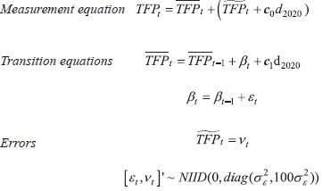
| (1) |
By adding the dummy variable to the first transition equation, we assume that the macroeconomic shock caused by the coronavirus pandemic affected the trend level of TFP (xxxxxxxxxx ) in 2020 (level shift). On the other hand, by adding the dummy variable to the measurement equation we take into account the effects of containment measures on the level of TFP that are temporary, i.e., the result of temporary supply constraints related to epidemiological measures.
The parameters with the dummy variables ( c0 i c1) were calibrated in such a way that the revised estimate of potential GDP meets the following criteria 30: (1) his-torical estimates – we preferred calibration in which revisions of historical potential output and total factor productivity were as small as possible (see figures 1 and 3), (2) the output gap is decomposed into demand and supply shock using the PACMAN semi-structural macroeconomic model 31 and the Phillips curve taking it into account that the implied output gap should be a major factor in explaining core inflation developments 32, and (3) the TFP growth rate returns to pre-pandemic levels in the long run. Namely, due to the uncertainty about the effects of the pandemic shock on the growth rate of potential GDP in the long run (which is significantly influenced by the estimated TFP growth rate in the long run), we preferred a calibration in which the long-run TFP growth rate converges to its pre-pandemic average (which amounts to 1% in the period from 2000 to 2019). 33
The potential GDP estimate which accounts for a structural break in the trend and cycle of TFP component is shown in figure 4. Data from the official CNB projection from December 2020 is based on relatively optimistic assumptions in terms of labour market and investment after the fall in 2020.
According to these estimates, potential GDP in 2020 will temporarily fall by about 1.6%, primarily due to a sharp decline in TFP caused by the coronavirus pandemic, whose negative contribution is estimated at 2.8%. This decline in potential GDP implies a negative output gap of 4.8%. In addition, this estimate implies that approximately 40% of the total decline in GDP in 2020 can be explained by supply shock, while the rest is attributed to a negative demand shock.
Figure 4Production factor contributions to potential output growth (in percentage, percentage points) DISPLAY Figure
The results suggests that the positive contribution to potential growth comes from labour and capital, with the positive contribution of capital in 2020 being lower than the positive contribution in 2019 primarily due to the contraction of investments in 2020. The positive contribution of labour to potential growth is comparable to that of the pre-pandemic year and is the result of still optimistic estimates related to the natural rate of unemployment.
In the long run, it is assumed that the potential growth rates of GDP and TFP will converge to their long-term average and amount to about 1.8% and 1%, respectively. The largest contribution to potential GDP growth could stem from capital due to optimistic forecasts of investments in the coming years related to EU funds and the reconstruction of Zagreb. On the other hand, the contribution of labour could be neutral in the long run, where the decline in working age population and working hours could be offset by a positive contribution to the decline in the natural unemployment rate and higher labour market participation.
As mentioned earlier, these are the results of one possible calibration of dummy variables (c0 i c1) from equation (1), in which we explained 40% of the total GDP decline in 2020 by supply shock and the rest by demand shock. However, by different calibration of these dummy variables, we were able to obtain significantly different estimates of potential growth and the output gap, as shown in figure 5.
Figure 5Potential growth and output gap estimated using different calibrations of the effect of the COVID-19 crisis on the trend and cycle component of TFP DISPLAY Figure
5 Output gap and capacity utilization rate
The previous two chapters have dealt with different potential GDP and the output gap estimation strategies, with special emphasis on adjustments made in the presence of an unprecedented structural break. It was shown that the results (i.e. estimates of potential growth and gap) are very sensitive to the choice of estimation strategy. Therefore, the obtained estimates should be continuously re-evaluated to make adequate real-time policy decisions. In that context, it will be useful to compare our preferred (benchmark) estimate with an alternative measure of the output gap such as capacity utilization rate, which is an indicator of the amount of economic slack in the industrial sector. Data are based on a survey of the firms within the manufacturing industry conducted and published by the European Commission. In this survey, manufacturing companies answer the question at what level of capacity they currently operate, expressed as a percentage of their total capacity, the ECB (2011b). Data for Croatia are available quarterly from the third quarter of 2008.
Figure 6Output gap and capacity utilization rate in Croatia (percentage) DISPLAY Figure
Figure 6 shows that the capacity utilization rate and the estimate of the output gap using the production function method are similar in their identification of the Croatian business cycle phases during the period 2009-2020. The European Commission’s November 2020 GDP gap estimate, which is also presented, shows similar behaviour. 34 After the prolonged period dominated by economic and public finance crises, the capacity utilization rate in Croatia began to grow significantly in 2013, indicating a somewhat faster start to the economic recovery than the output gap estimates suggested at the time. 35 Also, the European Commission’s assessment and capacity utilization rate signal a significant “overheating” of the economy just before the outbreak of the crisis. The CNB’s estimate points to somewhat milder “overheat” due to the estimation strategy, which aimed at minimal historical revisions. All three indicators recorded a sharp decline in 2020, with both output gaps hitting historic low levels, while the capacity utilization rate remained above the levels recorded during the last recession.
It should be noted that the capacity utilization is never revised, as is the case with most survey based indicators, while model estimates of the output gap are regularly revised (ECB, 2011b). An additional disadvantage of this indicator is that it applies only to the manufacturing sector, while the output gap applies to the whole economy. In addition, general problems with surveys are that firms may interpret questions differently and that most surveys have a limited base of answers (see Christiano, 1981). Regardless of these shortcomings, there is a high correlation between the capacity utilization rate and the output gap estimates in Croatia. Additionally, it seems that the adjustment of the potential GDP for structural break (which is described in detail in chapter 4.3) resulted in an output gap estimate that is in line with the capacity utilization indicator in 2020. 36
6 Concluding remarks and implications on economic policy
Measures imposed by governments to curb the spread of coronavirus are a unique example of temporary supply-side constraints. The question arises as to what extent these measures have affected potential GDP (ECB, 2020). Namely, as the potential GDP is an unobservable variable whose estimate is uncertain even in stable economic conditions, such a shock made the estimate of the potential GDP very challenging.
This paper describes and models the possible effects of the COVID-19 pandemic on Croatia’s potential GDP. The paper presents a conceptual framework for estimating potential GDP and points out the importance of potential GDP estimation for economic policy makers, especially concerning their stabilizing role in the economy. The paper points out the problems of estimating potential GDP in conditions of unprecedented macroeconomic shock and demonstrates these problems using four frequently used approaches to estimating potential GDP. The assessment of the effects of the pandemic crisis on potential GDP was followed by an analysis and explanations of the transmission channels through which epidemiological measures affected (and continue to affect) potential GDP within the production function-based approach. The paper pays special attention to the identification of the nature of the shock, i.e., the decomposition of the pandemic shock to the supply shock and the demand shock. In addition, the paper describes the implications of uncertainty regarding this decomposition because the latter has important implications for the output gap estimation.
Finally, the paper proposes a benchmark estimate of potential GDP in Croatia and addresses several possible ways 37 in which to estimate potential output in the con-text of the COVID-19 crisis. The benchmark estimation takes into account the ECB’s ( 2020) recommendations on the desirable properties of estimating potential GDP and the economic implications of the calibrated decomposition of the 2020 shock to supply and demand shock.
In addition, the paper presents an alternative estimate of the output gap in Croatia using alternative methodological approaches to estimate potential GDP and capacity utilization rate. Although our benchmark estimate of potential GDP is aligned with alternative business cycle indicators, it should be emphasized that the proposed estimate is preliminary given that the duration of the pandemic and pandemic-related government measures to combat the spread of the virus remains unknown.
Additionally, the paper indicates that measuring potential GDP is far from perfect. Whichever method is used, the results depend significantly on implicit assumptions that may or may not be valid. Some authors, such as Fontanari, Palumbo and Salvatori ( 2020) advocate a revision of the conceptual framework within which potential GDP is analyzed and measured. Namely, the most commonly used methods of estimating potential GDP generate results that are in line with the view of the cycle as short-term fluctuations in GDP around potential. However, the authors show that if the estimate of potential GDP is thought of as the level of GDP that can be achieved with full employment, then real GDP can remain below potential for decades. The authors assume that full employment is implicitly determined by the lowest unemployment rate ever achieved, which is in line with Okun’s proposals related to the target unemployment rate (Fontanari, Palumbo and Salvatori, 2020). Therefore, the authors believe that conventional methods generally underestimate potential GDP. If this is true, conventional methods also underestimate the negative output gap, i.e., overestimate the positive output gap. The implications for economic policies are clear. Economic policy makers will either underestimate the necessary expansion in bad economic times, either due to fiscal rules or fear of inflation, and overestimate the necessary restriction in (seemingly) better economic times.
In any case, the data on Croatian economy suggest that in 2020 there was a significant decline in potential GDP accompanied by a record large negative output gap. Developments related to the pandemic are uncertain, but a timely response from monetary and fiscal authorities is crucial at this time. Strong expansionary measures are a necessary condition for stabilizing the economy and its faster recovery, not only in the short, but probably also in the medium term.
Appendix
Appendix 1: Hodrick-Prescott filter
The univariate statistical filter introduced by Hodrick and Prescott (1981) separates the time series into a long-term trend  and a short-term cyclical component and a short-term cyclical component  minimizing the following function: minimizing the following function: 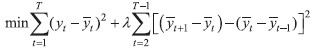 | (A.1.1) |
Appendix 2: Production function method
The estimation of potential growth and the output gap based on the production function method implicitly defines potential GDP as a level of production that can be achieved over a long period without excessive or insufficient use of existing production capacity, which implies the absence of price pressures. We define the production function as Cobb-Douglas with constant returns to scale: 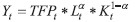 | (A2.1) |
To estimate the potential GDP, it is necessary to estimate the potential, i.e., long-term trend level of individual production factors and total factor productivity, and then the estimate of potential GDP is obtained from the equation of the production function.
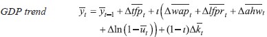
The labour factor is defined as the number of paid working hours in the economy
and is calculated using the following identity:
Lt = average hours worked per employeet * (1 – NAWRUt)
* participation ratet * working age populationt
The output gap is calculated as the difference between actual and potential GDP, expressed as a percentage of potential GDP.
Appendix 3: Multivariate filter
The structure of a simple multivariate filter used to estimate potential GDP in Croatia is based on Alichi et al. (2015).38 The model includes three core variables (real GDP, CPI inflation and unemployment rate). The annual data for Croatia are taken from Eurostat and the Croatian Bureau of Statistics. The model also includes real GDP growth forecasts five years ahead and one-year-ahead CPI inflation forecast. The forecasts should help identify the nature of the shocks (supply or demand).
Therefore, the complete database includes the Croatian National Bank’s published or unpublished GDP growth and CPI inflation forecasts. When no official CNB projections are available, GDP and inflation are projected using a simple autoregressive model. We assume that the last available GDP growth projection reflects the long-run growth rate of Croatia. Therefore, the last (three years ahead) CNB forecast is used as a four- and five-years-ahead forecast.
The following equations link the model’s core and the unobservable variables, the most important of which is potential GDP. The notation and equations presented here are identical to those in Alichi et al. ( 2015). The values of the parameters and the variances of the shocks are estimated using Bayesian techniques.
Output gap is defined as the deviation of the logarithm of the real GDP ( Yt) from the potential GDP  ![]() :  | (A3.1) |
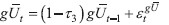
The output (real GDP) is a stochastic process comprised of three equations, each of which defines one shock type – potential output-level shock  potential output growth shock ( εGt) and output gap shock ( εγt). 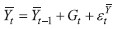 | (A3.2) |
 | (A3.3) |
 | (A3.4) |
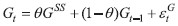
The level of potential output evolves according to potential growth ( Gt) and potential output-level shock. Potential growth is affected by the steady-state potential GDP growth rate ( GSS) and by the potential output growth shocks, which, depending on the value of θ, fade faster (low θ) or slower (high θ). GDP gap ( yt) is autoregressive process that is subject to output gap shocks which are perceived as demand shocks ![]() ( εγt).
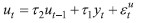
To help identify the three output shocks, a Phillips Curve equation for inflation is added, which links the evolution of the unobservable output gap ( yt) to observable data on inflation ( πt) according to the following process: 39 | (A3.5) |
Equations describing unemployment developments have been added to the model as these provide additional information for the output gap estimation:
 | (A3.6) |
 | (A3.7) |
 | (A3.8) |
 | (A3.9) |
In equation A3.6  is time varying non-accelerating inflation rate of unemployment (NAIRU) which is subject to shocks  and variation in the trend  which is itself also subject to shocks  This specification allows the natural unemployment rate (NAIRU) to deviate persistently from its equilibrium (steady-state) level.
The most important equation in this block specifies Okun’s law (equation A3.8) which links deviations of the observed unemployment rate ( Ut) from NAIRU  i output gap ( yt).
Core model equations are represented by equations A3.1 – A3.9, and these are enough to estimate potential GDP. However, extended version of the model allows us to make use of expected GDP growth (gCNBt+j) and inflation (πCNBt+j) (forecasts) which help to identify shocks and improve model’s forecasting performance at the end of the sample. 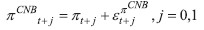 | (A3.10) |
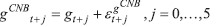 | (A3.11) |
Alichi et al. ( 2015) emphasize that in practice the estimated variances of errors  in equations A3.10 and A3.11 allow forecasts to influence, but not completely replace, model expectations (especially at the very end of the sample). However, the authors suggest that this information can significantly influence historical estimates of potential GDP and the output gap.
Table A3.1Data sources DISPLAY Table
Appendix 4: Multivariate filter combined with production function
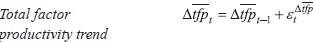
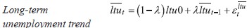
The structure of the multivariate unobserved components model used in this paper was described in detail by Tóth (2021). It is a state-space model based on the production function and on some well-known economic relations such as Okun’s law and the Phillips curve (the latter can be turned on or off arbitrarily). In the model, the six underlying observable variables are decomposed into their trend and cycle component (real GDP, unemployment rate, participation rate, working hours, core inflation, and wage growth). The trend components of these variables serve as input variables for the production function. In addition, the model uses three additional observable variables (capital, working age population and long-term unemployment rate) that are not decomposed into trend and cycle, as it is standard in the literature. The equations of the observed values – measurement equations – are given as follows: 
| (A4.1) |

| (A4.2) |

| (A4.3) |

| (A4.4) |

| (A4.5) |

| (A4.6) |

| (A4.7) |

| (A4.8) |
 | (A4.9) |

| (A4.10) |
| (A4.11) |

| (A4.12) |

| (A4.13) |
 | (A4.14) |

| (A4.15) |
| (A4.16) |
 | (A4.17) |
| (A4.18) |

| (A4.19) |
 | (A4.20) |
| (A4.21) |
The unemployment rate, as mentioned earlier, is also decomposed into its trend and cycle component, and then its cycle is linked to the output gap under Okun’s law. The unemployment trend (i.e., NAIRU) is not a stationary time series and takes into account changes in the long-term unemployment rate.

| (A4.22) |

| (A4.23)
|

| (A4.24) |

| (A4.25)
|
Wage growth (compensation per employee) is disaggregated in a similar way. The Phillips wage curve links the wage growth gap with the unemployment gap, and the wage growth trend is assumed to be the sum of the inflation trend and the labour productivity growth trend.

| (A4.26) |

| (A4.27) |
The model is evaluated in its state-space form using the Bayesian approach. The evaluation of model parameters and unobservable variables is performed using a Kalman filter.
Table A4.1Data sources DISPLAY Table
Appendix 5: Comparison of our benchmark estimate of the potential GDP with the European Commission's
Differences in the estimates of potential GDP growth provided by the European Commission and those in this paper arise from different technical assumptions related to the potential GDP components systematically shown in table A5.1. The majority of differences arise from differences in the TFP and labour market-related variables. The contributions of individual components to potential GDP growth are shown in figure A5.1. and quantify these differences. The estimate of the contribution of the TFP to the growth of the potential GDP of the EC (left side of figure A5.1) is significantly lower than our estimate (right side of figure A5.1). On the other hand, we assess the neutral contribution of labour factors to the potential GDP growth rate in 2022 and 2023, while the European Commission implies a positive contribution of labour to potential GDP growth in 2022, followed by a negative 2023.
Table A5.1Assumptions used to calculate potential GDP DISPLAY Table
Figure A5.1Comparison of contributions to potential GDP growth, EC – left, ours – right (in percentage, percentage points) DISPLAY Figure
At the same time, the estimates of the European Commission from December 2020 show large historical revisions of the total factor productivity and labour factors in relation to the estimate from December 2019, which is difficult to explain. The right-hand graph in figure A5.2 shows the effect of the adjustment for structural break in 2020 on our estimate of potential GDP in that year (red line shows the estimate with structural break, and the black solid line without structural break), as well as the previous estimate of potential GDP from 2019. It can be seen that our estimate of potential GDP would have the same undesirable features (significant revision of potential GDP, and thus the output gap, shown in the past in figure A5.2.) if it were not adjusted for structural fracture in 2020 (black solid line and black dashed line begin to diverge as early as 2015).
In figure A5.3 estimates of the growth rates of potential GDP given by the European Commission and those in this paper are compared. The traditionally more pessimistic estimate of the potential growth of the European Commission in the long run is clearly visible (0.4% vs 1.8%). The European Commission’s estimate of potential growth is also seen to be significantly lower (0.4% vs. 1.1% from the 2019Q4 estimate), while ours has not significantly revised potential long-term GDP growth rate. The reason for this is the difficulty in assessing the effect of the COVID-19 crisis on growth in the long run, with arguments presented for both lower and higher potential growth rates in the long run. In the short run, it can be seen that estimates of potential growth in the past have been less revised in our estimate of structural break in 2020 (red line in the right-hand chart of A5.3). In 2020, it can be seen that our estimate attributes most of the decline to a temporary supply shock, which also results in smaller revisions of potential GDP in the past. Of course, the same conclusions apply to the revision of the historical output gap shown in figure A5.4.
Figure A5.2Comparison of the potential GDP estimate from December 2020 and December 2019, EC – left, our estimate – right (HRK bn) DISPLAY Figure Figure A5.3Comparison of the potential growth estimate from December 2020 and December 2019, EC – left, our estimate – right (percentage) DISPLAY Figure Figure A5.4Comparison of the output gap (percentage) DISPLAY Figure
Notes
* All views presented in this paper are the authors’ own and do not necessarily reflect the official position of the Croatian National Bank. The authors would like to thank two anonymous reviewers and colleagues from the Croatian National Bank for their useful suggestions. This article will also be published as Croatian National Bank Working paper.
1 For a detailed overview of the ideas and development of the methodology related to the separation of the trend and cycle of GDP, see for example Cerra, Fatas and Saxena (2020).
2 Earlier thoughts on economic cycles and fluctuations did not address their practical identification in a modern sense (see in more detail in Beveridge and Nelson, 1981).
3 One of the main purposes of the book was to list the methods of measuring the cyclical behaviour of the economy developed by the NBER and their practical application in identifying the turning points of the business cycle.
4 Despite the fact that business cycle identification today uses methods that over time deviated from the approaches proposed by Burns and Mitchell (1946), the conceptual framework they developed can still be recognized today in various methods of identifying business cycle turning points. One of the first researches in which the turning points of the business cycle in Croatia were identified, using three different methods, was conducted by Krznar (2011a).
5 According to Beveridge and Nelson (1981), one of the popular methods identified cycles as output deviations from a deterministically determined trend where the trend was most often shown as (most commonly polynomial) function of time (see for example Fellner, 1956), which is a very strong assumption. Although in Friedman (1957) when dividing income into permanent and transient components, the permanent (trend) component was not deterministic, it implied "fairly strong initial assumptions about the stochastic properties of the permanent component" (Beveridge and Nelson, 1981). Two alternative cycle measurement methods were developed by Mintz (1969; 1972), one of which defined the trend using a centred 75-month moving average, and the other focused on the analysis of fluctuations in rate of change. On the technical side, the problem arises towards the end of the sample in which future observations of the series under observation are not available (for a more detailed critique, see Beveridge and Nelson (1981)).
6 Arčabić (2018) analyses theoretically and empirically the separation of trend and cycle components of GDP in order to identify the nature of shocks (supply or demand) in selected post-transition countries. The paper shows how demand shocks are dominant in explaining the business cycles of almost all post-transition countries, which is in strong contrast to the conclusions of the real business cycle theory.
7 See for example Blanchard and Quah (1989).
8 Although this is the dominant conceptual view of potential GDP, different estimation methods often start from different definitions of potential GDP (see Chapter 3).
9 Depending on the estimation method, this problem may be more or less pronounced. The problem is most pronounced with (often symmetrical) two-sided filters such as HP filters (Jovičić, 2017) in which variable shifts (e.g., GDP in the case of univariate filter estimation) are used forward and backward to estimate potential GDP (historical and future data) where no data on future trends are available at the end of the sample.
10 The consequences of these two problems for the conduct of economic policies are beyond the scope of this paper.
11 Also, these new data cause (sometimes significant) revisions of historical estimates of potential GDP, which is certainly not a desirable feature of potential GDP estimates from the perspective of theoretical assumptions and desirable properties of potential GDP estimates (see Chapter 4).
12 For a more detailed explanation and demonstration of these properties, see Chapter 3.
13 See Jovičić (2017) for a detailed overview of differences in estimates of the cyclically-adjusted budget balance depending on the method used to estimate potential GDP.
14 Some authors (see for example Heimberger, 2020) believe that the underestimation of the negative output gap has contributed to the deepening and prolongation of the consequences of the 2008/2009 global financial crisis due to excessive emphasis on the need for fiscal consolidation in countries with unfavourable fiscal position (indicated by the cyclically-adjusted budget balance).
15 Hysteresis is easiest to explain by the impact of crises on the labour market. As the unemployment rate rises during the crisis, part of the labour force becomes inactive and deprives human capital during inactivity. The longer the period of inactivity, the more difficult it is to return to the labour market, which leads to an increase in structural unemployment, and thus to a long-term loss of productive resources that reduce potential GDP. In addition, numerous rigidities in the labour market can also slow down adjustment towards equilibrium in this market. Due to slow adjustment, changes in the unemployment rate become persistent and may have long-term consequences for potential GDP.
16 In that part in which it does not distort the economic balance.
17 Appendices 1-4 give a more detailed description of all four methodological approaches for estimating potential GDP.
18 A similar analysis of different ways of estimating potential GDP was conducted by Jovićić (2017).
19 Although both institutions use the production function method, estimates of potential GDP differ. The differences arise from the way the trend and cycle components of production factors are estimated (primarily those related to labour), from using different indicators (data) for production factors of production and finally from using different projections of production factors in the long run (see Appendix 5).
20 Alichi et al. (2015) showed that, although real-time estimates of potential GDP are quite uncertain, this approach gives more adequate estimates of potential GDP compared to univariate statistical filters.
21 See Jovičić (2017) for a more detailed analysis of the sensitivity of different potential GDP estimates to the end-of-sample bias based on Croatian data.
22 Arčabić (2018) gives a detailed overview of theoretical concepts and methodological approaches for separating the cycle and trend component of GDP, in the context of supply and demand shocks. The analysis includes Croatia, and the author shows that in Croatia, fluctuations in GDP in the past were dominated by demand shocks.
23 The authors conducted the analysis for the US, UK, euro area and Japan.
24 The red and blue lines start to diverge from 2015, but their differences become significant after 2016.
25 The same thing happened with the estimate of potential GDP published by the European Commission when comparing estimates of potential GDP in autumn 2019 (see European Commission, 2019) and autumn 2020 (see European Commission, 2020). The EC's estimates are compared with the estimates in this paper and presented in Appendix 5.
26 In the crisis of 2008/2009 this transmission mechanism has been strong in European Union countries (see, for example, the ECB, 2012).
27 See for example Caballero and Hammour (1994).
28 As explained earlier, this is a consequence of the introduced government support measures in the labour market, while in the case of capital the effect is reduced due to investments in earthquake-affected areas.
29 Given that this is a residual category, the estimated TFP, among other things, contains errors in measuring production factors and the degree of utilization of existing capacity in the economy. However, we do not have a sufficiently long reference measure for the degree of capacity utilization in Croatia that we could use to estimate potential GDP. Also, this is why the greatest short-term effect of the pandemic shock can be attributed TFP, because measures to combat the spread of the pandemic have had the greatest impact on the degree of utilization of existing physical and human capacity in the economy.
30 The criteria are in line with the ECB's (2020) recommendations on the desirable features of estimating potential GDP.
31 See Nadoveza Jelić and Ravnik (2021).
32 The adjustment was performed using the PACMAN macroeconomic model and projections of headline and core inflation with respect to alternative output gap sizes in the Phillips curve. The ultimate goal was for the selected calibration to result in an output gap that would align the 2020 inflation with the HNB's official December 2020 inflation projection.
33 Data on TFP for 2009 was not included due to an extremely high drop of approximately 8%.
34 The differences from the CNB's estimate are explained in more detail in Annex 5.
35 This indication of the earlier beginning of the economic “overheating” would signal to policymakers the need to introduce restrictive measures quicker due to the potential inflationary pressures.
36 Nelson (2008) and Morley and Panovska (2020) argue that the correlation between the appropriately estimated output gap and the one-year-ahead real GDP growth rate should be negative. The intuition behind this argument is that as the economy returns to its long-term trend when the output gap is positive we should expect future GDP growth rates to be below average. Correlations between output gap measures presented in Figure 6 and the one-year-ahead real GDP growth rate were calculated to verify if these measures satisfy this intuition. The correlations obtained verified that all three measures of the output gap are negatively correlated with the future GDP growth rate.
37 That is, we propose and argue one basic calibration of the possible countless calibrations of the decomposition of GDP decline in 2020 to supply and demand shock.
38 The code is available on the personal page of the co-author of the paper Douglas Laxtonl.
39 Several studies question the existence of the Phillips curve in Croatia; see for example Krznar ( 2011b), Botrić ( 2012), Jovičić and Kunovac ( 2017). When estimating the potential GDP in Croatia using a simple multivariate filter based on Alichi et al. ( 2015), we also try it with the inactive mechanism of the Phillips curve. In this case, equation P3.5 is simply given by: πt= πt-1. However, since the results do not differ significantly in the two alternative model specifications, we present the results with the active Phillips curve. On the other hand, when estimating potential GDP using the unobserved components model the results differ significantly and, therefore, we presume an inactive mechanism of the Phillips curve.
* All views presented in this paper are the authors’ own and do not necessarily reflect the official position of the Croatian National Bank. The authors would like to thank two anonymous reviewers and colleagues from the Croatian National Bank for their useful suggestions. This article will also be published as Croatian National Bank Working paper.
1 For a detailed overview of the ideas and development of the methodology related to the separation of the trend and cycle of GDP, see for example Cerra, Fatas and Saxena ( 2020).
2 Earlier thoughts on economic cycles and fluctuations did not address their practical identification in a modern sense (see in more detail in Beveridge and Nelson, 1981).
3 One of the main purposes of the book was to list the methods of measuring the cyclical behaviour of the economy developed by the NBER and their practical application in identifying the turning points of the business cycle.
4 Despite the fact that business cycle identification today uses methods that over time deviated from the approaches proposed by Burns and Mitchell ( 1946), the conceptual framework they developed can still be recognized today in various methods of identifying business cycle turning points. One of the first researches in which the turning points of the business cycle in Croatia were identified, using three different methods, was conducted by Krznar ( 2011a).
5 According to Beveridge and Nelson ( 1981), one of the popular methods identified cycles as output deviations from a deterministically determined trend where the trend was most often shown as (most commonly polynomial) function of time (see for example Fellner, 1956), which is a very strong assumption. Although in Friedman ( 1957) when dividing income into permanent and transient components, the permanent (trend) component was not deterministic, it implied "fairly strong initial assumptions about the stochastic properties of the permanent component" (Beveridge and Nelson, 1981). Two alternative cycle measurement methods were developed by Mintz ( 1969; 1972), one of which defined the trend using a centred 75-month moving average, and the other focused on the analysis of fluctuations in rate of change. On the technical side, the problem arises towards the end of the sample in which future observations of the series under observation are not available (for a more detailed critique, see Beveridge and Nelson ( 1981)).
6 Arčabić ( 2018) analyses theoretically and empirically the separation of trend and cycle components of GDP in order to identify the nature of shocks (supply or demand) in selected post-transition countries. The paper shows how demand shocks are dominant in explaining the business cycles of almost all post-transition countries, which is in strong contrast to the conclusions of the real business cycle theory.
7 See for example Blanchard and Quah ( 1989).
8 Although this is the dominant conceptual view of potential GDP, different estimation methods often start from different definitions of potential GDP (see Chapter 3).
9 Depending on the estimation method, this problem may be more or less pronounced. The problem is most pronounced with (often symmetrical) two-sided filters such as HP filters (Jovičić, 2017) in which variable shifts (e.g., GDP in the case of univariate filter estimation) are used forward and backward to estimate potential GDP (historical and future data) where no data on future trends are available at the end of the sample.
10 The consequences of these two problems for the conduct of economic policies are beyond the scope of this paper.
11 Also, these new data cause (sometimes significant) revisions of historical estimates of potential GDP, which is certainly not a desirable feature of potential GDP estimates from the perspective of theoretical assumptions and desirable properties of potential GDP estimates (see Chapter 4).
12 For a more detailed explanation and demonstration of these properties, see Chapter 3.
13 See Jovičić ( 2017) for a detailed overview of differences in estimates of the cyclically-adjusted budget balance depending on the method used to estimate potential GDP.
14 Some authors (see for example Heimberger, 2020) believe that the underestimation of the negative output gap has contributed to the deepening and prolongation of the consequences of the 2008/2009 global financial crisis due to excessive emphasis on the need for fiscal consolidation in countries with unfavourable fiscal position (indicated by the cyclically-adjusted budget balance).
15 Hysteresis is easiest to explain by the impact of crises on the labour market. As the unemployment rate rises during the crisis, part of the labour force becomes inactive and deprives human capital during inactivity. The longer the period of inactivity, the more difficult it is to return to the labour market, which leads to an increase in structural unemployment, and thus to a long-term loss of productive resources that reduce potential GDP. In addition, numerous rigidities in the labour market can also slow down adjustment towards equilibrium in this market. Due to slow adjustment, changes in the unemployment rate become persistent and may have long-term consequences for potential GDP.
16 In that part in which it does not distort the economic balance.
17 Appendices 1-4 give a more detailed description of all four methodological approaches for estimating potential GDP.
18 A similar analysis of different ways of estimating potential GDP was conducted by Jovićić ( 2017).
19 Although both institutions use the production function method, estimates of potential GDP differ. The differences arise from the way the trend and cycle components of production factors are estimated (primarily those related to labour), from using different indicators (data) for production factors of production and finally from using different projections of production factors in the long run (see Appendix 5).
20 Alichi et al. ( 2015) showed that, although real-time estimates of potential GDP are quite uncertain, this approach gives more adequate estimates of potential GDP compared to univariate statistical filters.
21 See Jovičić ( 2017) for a more detailed analysis of the sensitivity of different potential GDP estimates to the end-of-sample bias based on Croatian data.
22 Arčabić ( 2018) gives a detailed overview of theoretical concepts and methodological approaches for separating the cycle and trend component of GDP, in the context of supply and demand shocks. The analysis includes Croatia, and the author shows that in Croatia, fluctuations in GDP in the past were dominated by demand shocks.
23 The authors conducted the analysis for the US, UK, euro area and Japan.
24 The red and blue lines start to diverge from 2015, but their differences become significant after 2016.
25 The same thing happened with the estimate of potential GDP published by the European Commission when comparing estimates of potential GDP in autumn 2019 (see European Commission, 2019) and autumn 2020 (see European Commission, 2020). The EC's estimates are compared with the estimates in this paper and presented in Appendix 5.
26 In the crisis of 2008/2009 this transmission mechanism has been strong in European Union countries (see, for example, the ECB, 2012).
27 See for example Caballero and Hammour ( 1994).
28 As explained earlier, this is a consequence of the introduced government support measures in the labour market, while in the case of capital the effect is reduced due to investments in earthquake-affected areas.
29 Given that this is a residual category, the estimated TFP, among other things, contains errors in measuring production factors and the degree of utilization of existing capacity in the economy. However, we do not have a sufficiently long reference measure for the degree of capacity utilization in Croatia that we could use to estimate potential GDP. Also, this is why the greatest short-term effect of the pandemic shock can be attributed TFP, because measures to combat the spread of the pandemic have had the greatest impact on the degree of utilization of existing physical and human capacity in the economy.
30 The criteria are in line with the ECB's ( 2020) recommendations on the desirable features of estimating potential GDP.
31 See Nadoveza Jelić and Ravnik ( 2021).
32 The adjustment was performed using the PACMAN macroeconomic model and projections of headline and core inflation with respect to alternative output gap sizes in the Phillips curve. The ultimate goal was for the selected calibration to result in an output gap that would align the 2020 inflation with the HNB's official December 2020 inflation projection.
33 Data on TFP for 2009 was not included due to an extremely high drop of approximately 8%.
34 The differences from the CNB's estimate are explained in more detail in Annex 5.
35 This indication of the earlier beginning of the economic “overheating” would signal to policymakers the need to introduce restrictive measures quicker due to the potential inflationary pressures.
36 Nelson ( 2008) and Morley and Panovska ( 2020) argue that the correlation between the appropriately estimated output gap and the one-year-ahead real GDP growth rate should be negative. The intuition behind this argument is that as the economy returns to its long-term trend when the output gap is positive we should expect future GDP growth rates to be below average. Correlations between output gap measures presented in Figure 6 and the one-year-ahead real GDP growth rate were calculated to verify if these measures satisfy this intuition. The correlations obtained verified that all three measures of the output gap are negatively correlated with the future GDP growth rate.
37 That is, we propose and argue one basic calibration of the possible countless calibrations of the decomposition of GDP decline in 2020 to supply and demand shock.
39 Several studies question the existence of the Phillips curve in Croatia; see for example Krznar ( 2011b), Botrić ( 2012), Jovičić and Kunovac ( 2017). When estimating the potential GDP in Croatia using a simple multivariate filter based on Alichi et al. ( 2015), we also try it with the inactive mechanism of the Phillips curve. In this case, equation P3.5 is simply given by: πt= πt-1. However, since the results do not differ significantly in the two alternative model specifications, we present the results with the active Phillips curve. On the other hand, when estimating potential GDP using the unobserved components model the results differ significantly and, therefore, we presume an inactive mechanism of the Phillips curve.
Disclosure statement
All authors state that they do not have any financial or other substantive conflict of interest.
References
Alichi, A. [et al.], 2015. Multivariate Filter Estimation of Potential Output for the Euro Area and the United States. IMF Working Paper, No. 15/253.
Beveridge, S. and Nelson, C., 1981. A new approach to decomposition of economic time series into permanent and transitory components with particular attention to measurement of the 'business cycle'. Journal of Monetary Economics, 7(2), pp. 151-174 [ CrossRef]
Burns, A. F. and Mitchell, W. C., 1946. Measuring Business Cycles. Studies in business cycles. Cambridge, MA: NBER.
Fellner, W., 1956. Trends and cycles in economic activity. New York: Henry Holt.
Fontanari, C., Palumbo, A. and Salvatori, C., 2020. Potential Output in Theory and Practice: A Revision and Update of Okun's Original Method. Structural Change and Economic Dynamics, 54, pp. 247-266 [ CrossRef]
Friedman, M., 1957. A theory of the consumption function. Princeton: Princeton University Press.
Hodrick, R. J. and Prescott, E., 1997. Postwar business cycles: an empirical investigation. Journal of Money, Credit, and Banking, pp. 1-16 [ CrossRef]
Jovičić, G. and Kunovac, D., 2017. What is Driving Inflation and GDP in a Small European Economy: The Case of Croatia. CNB Working Papers, W-49.
Koopmans, T. C., 1947. Measurement Without Theory. The Review of Economics and Statistics, 29(3), pp. 161-172 [ CrossRef]
Kydland, F. E. and Prescott, E. C., 1982. Time to Build and Aggregate Fluctuations. Econometrica: Journal of the Econometric Society, 50(6), pp. 1345-1370 [ CrossRef]
Mintz, I., 1969. Dating postwar business cycles. New York: NBER.
Mintz, I., 1972. Dating American growth cycles. In: V. Zarnowitz. The Business Cycle Today, New York: NBER, pp. 39-88.
Nadoveza Jelić, O. and Ravnik, R., 2021. Introducing Policy Analysis Croatian MAcroecoNometric Model (PACMAN). CNB Survey, S-41.
Nelson, C. R., 2008. The Beveridge–Nelson decomposition in retrospect and prospect. Journal of Econometrics, 146(2), pp. 202-206 [ CrossRef]
Solow, R. M., 1956. A Contribution to the Theory of Economic Growth. The Quarterly Journal of Economics, 70(1), pp. 65-94 [ CrossRef]
Tóth, M., 2021. A Multivariate Unobserved Components Model to Estimate Potential Output in the Euro Area: A Production Function Based Approach. ECB Working Paper, No. 2523.
Alichi, A. [et al.], 2015. Multivariate Filter Estimation of Potential Output for the Euro Area and the United States. IMF Working Paper, No. 15/253.
Beveridge, S. and Nelson, C., 1981. A new approach to decomposition of economic time series into permanent and transitory components with particular attention to measurement of the 'business cycle'. Journal of Monetary Economics, 7(2), pp. 151-174 [ CrossRef]
Burns, A. F. and Mitchell, W. C., 1946. M easuring Business Cycles. Studies in business cycles. Cambridge, MA: NBER.
Fellner, W., 1956. Trends and cycles in economic activity. New York: Henry Holt.
Fontanari, C., Palumbo, A. and Salvatori, C., 2020. Potential Output in Theory and Practice: A Revision and Update of Okun's Original Method. Structural Change and Economic Dynamics, 54, pp. 247-266 [ CrossRef]
Friedman, M., 1957. A theory of the consumption function. Princeton: Princeton University Press.
Hodrick, R. J. and Prescott, E., 1997. Postwar business cycles: an empirical investigation. Journal of Money, Credit, and Banking, pp. 1-16 [ CrossRef]
Jovičić, G. and Kunovac, D., 2017. What is Driving Inflation and GDP in a Small European Economy: The Case of Croatia. CNB Working Papers, W-49.
Koopmans, T. C., 1947. Measurement Without Theory. The Review of Economics and Statistics, 29(3), pp. 161-172 [ CrossRef]
Kydland, F. E. and Prescott, E. C., 1982. Time to Build and Aggregate Fluctuations. Econometrica: Journal of the Econometric Society, 50(6), pp. 1345-1370 [ CrossRef]
Mintz, I., 1969. Dating postwar business cycles. New York: NBER.
Mintz, I., 1972. Dating American growth cycles. In: V. Zarnowitz. The Business Cycle Today, New York: NBER, pp. 39-88.
Nadoveza Jelić, O. and Ravnik, R., 2021. Introducing Policy Analysis Croatian MAcroecoNometric Model (PACMAN). CNB Survey, S-41.
Nelson, C. R., 2008. The Beveridge–Nelson decomposition in retrospect and prospect. Journal of Econometrics, 146(2), pp. 202-206 [ CrossRef]
Solow, R. M., 1956. A Contribution to the Theory of Economic Growth. The Quarterly Journal of Economics, 70(1), pp. 65-94 [ CrossRef]
Tóth, M., 2021. A Multivariate Unobserved Components Model to Estimate Potential Output in the Euro Area: A Production Function Based Approach. ECB Working Paper, No. 2523.
|


