|
|
|
Abstract
The widening fiscal deficits and the increase of public debt triggered by the COVID-19 crisis suggest that fiscal policy makers will have to engage in substantial fiscal consolidation in order to stabilize public finances in the mid run. However, the implementation of a fiscal consolidation package, if it is not properly designed, can be detrimental for growth and even lead to a self-defeating outcome. In order to avoid this undesirable scenario, fiscal policy makers should rely on growth-friendly consolidation packages. The design of growth-friendly fiscal consolidation packages requires an understanding of the size of multipliers of different fiscal instruments. Thus, in this paper we provide the first deeper insights into the size of model-based disaggregated fiscal multipliers in Croatia. For this purpose, we have built a semi-structural macro-fiscal model of the Croatian economy and used Croatia’s experience during the fiscal consolidation episode under the excessive deficit procedure (EDP) to retrieve fiscal multipliers, analyse the design of the policy package and provide model-based evaluation of the macroeconomic effects of this consolidation episode. Our results indicate that the fiscal consolidation implemented during the EDP was not growth-friendly and that it was partially self-defeating. We hope that our results can help fiscal policy makers to avoid similar policy mistakes in future fiscal consolidations.
Keywords: fiscal consolidation; fiscal multipliers; Croatia; economic modelling
JEL: E62, E12, C50
1 Introduction
The Covid-19 pandemic has prompted governments around the world to implement large fiscal stimulus packages in order to mitigate the economic costs of this global shock. Discretionary fiscal actions led to a structural increase of budget expenditures (e.g. subsidies to companies and transfers to households) and a fall in revenues (e.g. tax reliefs), thus widening fiscal deficits. The fall in economic activity, mostly triggered by the lockdowns imposed, has put additional pressure on fiscal balances through a mechanism of automatic stabilizers. These developments will result in a strong increase of public debt in both absolute and relative terms.
The deteriorating fiscal balances in 2020 suggest that fiscal policy makers will have to make a substantial fiscal effort to consolidate public finances and stabilize public debt dynamics in the mid run. 1 This is especially important for Croatia on its path towards euro adoption. However, the implementation of fiscal consolidation packages, if not properly designed, could be detrimental for growth and thus even lead to self-defeating fiscal consolidation efforts. More precisely, poorly designed fiscal consolidation packages could additionally increase the public-debt-to-GDP ratio if the effects of a policy-induced fall in GDP 2 outweigh the effect of fiscal adjustment (Gros and Maurer,  2012 2012; Eyraund and Webber, 2013; Boussard, de Castro and Salto, 2013).
That is why fiscal policy makers should rely on growth-friendly fiscal consolidation packages. The basic idea behind growth-friendly fiscal consolidations is to design a fiscal consolidation package that ensures an improvement of fiscal balances, while minimizing negative short-term effects on growth (Cournède, Goujard and Pina, 2013). To put it differently, growth-friendly consolidation packages should be based on fiscal instruments with low fiscal multipliers as they could ensure the required fiscal effort with low economic costs.
The design of growth-friendly consolidation packages requires deep understanding of fiscal policy transmission mechanisms and knowledge about the size of fiscal multipliers of different fiscal instruments, i.e. so-called “disaggregated” fiscal multipliers (e.g. Boussard, de Castro and Salto, 2013; Cortuk, 2013). Thus, the key goal of this paper is to provide the first detailed insights into fiscal policy transmission mechanisms and the size of disaggregated fiscal multipliers in Croatia. Data on disaggregated fiscal multipliers can help fiscal policy makers in designing growth-friendly fiscal consolidation packages in the future.
Estimates of fiscal multipliers in Croatia have so far been exclusively based on vector autoregression methodology (VAR) (Šimović and Deskar-Škrbić, 2013; Grdović Gnip, 2014; 2015; Deskar-Škrbić and Šimović, 2017). Although the VAR-based approach to the estimation of fiscal multipliers dominates fiscal literature, it does not allow a comprehensive analysis of the complex transmission mechanisms of fiscal policy and offers a limited framework for the analysis of macroeconomic effects of different fiscal policy instruments and feedbacks from macroeconomic to fiscal variables. This kind of analysis requires a more modeloriented approach.
References to model-based evaluation of the macroeconomic effects of fiscal policy in Croatia are scarce. To our knowledge there are only three papers investigating the effects of fiscal policy through the lenses of economic models on the macro level, 3 but only for one fiscal instrument. Nadoveza, Sekur and Beg ( 2016) use the computable general equilibrium (CGE) model to analyse the macroeconomic effects of changes in the income tax burden. Deskar-Škrbić ( 2018) calibrates a small-scale dynamic stochastic general equilibrium (DSGE) model to simulate the effects of a government consumption shock on the Croatian economy. Bokan and Ravnik ( 2018) present the Croatian National Bank’s quarterly projection model (QPM) and simulate the effects of a change in the structural deficit.
This paper seeks to fill this gap in the literature by building and introducing for the first time a small semi-structural macro-fiscal model of the Croatian economy. This model allows us to retrieve disaggregated fiscal multipliers by comparing the realizations of macroeconomic variables in the no policy change and policy change scenarios, for different fiscal instruments. In addition, this model allows us to investigate the feedback from policy-induced changes in macroeconomic variables to fiscal balances and public debt. However, we want to emphasize that the model that we propose is not on a large enough scale to be able to capture all the relevant macroeconomic relations and the purpose of this model is not to describe the Croatian economy in detail but to give a basic framework for the analysis of the effects of fiscal policy. In addition, the proposed model (like other models in this class) is faced with various methodological limitations that we explain in detail in the main text.
The key challenge in the estimation of fiscal multipliers is to find episodes of exogenous changes in fiscal instruments, i.e. changes that are not directly related to business cycle developments. 4 However, Croatia’s recent experience during the excessive deficit procedure (EDP) from 2014 to 2016 offers a capacious framework for the analysis in this sense. The EDP fiscal consolidation episode is interesting, as the fiscal authorities implemented a series of structural fiscal measures. 5 These measures were reported in a transparent way and subjected to continuous post-hoc evaluations by the Commission. This fact enables a precise identification of structural measures that were not only announced by policy makers but actually implemented. In addition, fiscal policy actions were dominantly motivated by the supranational policy pressure under the EDP framework. In this sense, the implemented fiscal measures can be seen as exogenous, i.e. not directly related to the business cycle (Cugnasca and Rother, 2015; Górnicka et al., 2018).
Thus, in this paper we use these structural measures as input for our model and calculate the disaggregated fiscal multipliers for different revenue-side and expenditure-side fiscal instruments. Then, we use these findings to analyse whether the EDP fiscal consolidation episode was growth-friendly. Our results show that, although the consolidation was successful in terms of fiscal outcomes, the implemented fiscal package was not growth-friendly and the consolidation was partially self-defeating. In our counter-factual scenario, if our proposal for a growth-friendly fiscal consolidation package had been adopted, recession in Croatia would have ended as early as 2014, while public-debt-to GDP ratio would at the end of the consolidation period have been lower than it actually was. We hope that our findings can help fiscal policy makers to avoid similar mistakes in future fiscal consolidation episodes.
The paper is structured as follows. After the introduction, section 2 provides a brief literature review, with the focus on the literature on fiscal consolidations and the macroeconomic effects of fiscal policy. In section 3, we analyse the main characteristics of the EDP fiscal consolidation strategy and fiscal outcomes. In section 4, we present the structure of our small-scale semi-structural macro-fiscal model of the Croatian economy. In section 5, we present the main empirical results. The paper ends with the conclusion.
2 Conceptual framework of the analysis
In this paper, we build on two inter-related strands of the literature. First, we analyse the literature on fiscal consolidations. This strand of literature provides an analytical framework for understanding the key characteristics of the EDP fiscal consolidation episode in Croatia. Second, we present the literature on the evaluation of the macroeconomic effects of fiscal policy in different methodological frameworks. This strand of the literature helps us to explain and position the methodological approach adopted in this paper more effectively.
Fiscal consolidations The definition of fiscal consolidation mostly used in the literature is the improvement of a primary structural fiscal balance by 1.5pp of GDP in a single year (“cold shower” or “front-loaded”) or an improvement of at least 1.5pp of GDP in three years, with no annual deterioration larger than 0.5pp (“gradual consolidation” or “back-loaded”). This definition was first used in a seminal paper by Alesina and Perotti ( 1997) and later in the influential paper by Alesina and Ardagna ( 2010). Different institutions, such as the European Commission (e.g. Barrios, Langedijk and Pench, 2010) or the IMF (e.g. Escolano et al., 2014) also accept this definition.
Besides the definition of fiscal consolidation, the literature also offers measurable criteria for the identification of successful fiscal consolidation episodes. According to Alesina and Perotti ( 1995) and Barrios, Langedijk and Pench ( 2010), a fiscal consolidation episode can be labelled successful if three years after the start of consolidation the debt to GDP ratio is 5pp lower than it was at the beginning of the consolidation. Alternatively, the fiscal consolidation episode is successful if the cumulative improvement of the public debt-to-GDP ratio during the consolidation period is greater than 4.5pp (Alesina and Ardagna, 2010).
In this context, there is abundant literature on the key factors that affect the success of fiscal consolidations. Barrios, Langedijk and Pench ( 2010) conclude that the probability of achieving a successful consolidation reduces if a front-loading strategy is undertaken when the economy is experiencing a slowdown. A backloading strategy has the advantage of giving the economy more time to recover but raises uncertainty and it is considered inferior to a front-loaded approach if the debt is high and there are financial market pressures. As for the composition of consolidation measures, the literature shows that expenditure-based consolidations appear to be more effective in stabilizing debt than those that are revenuebased (e.g. Alesina and Perotti, 1995; von Hagen, Hallett and Strauch, 2002; Guichard et al., 2007; Alesina and Ardagna, 2010; Barrios, Langedijk and Pench, 2010, Alesina et al., 2017). This is mostly explained by the fact that consolidation policies based on increases in revenues (e.g. tax hikes) suggest a lack of political will for structural reforms. Nonetheless, revenue-based consolidations can also be effective, if there is room to increase the revenue-to-GDP ratio, in particular if the revenue types that are less harmful for growth (such as user fees, environmental taxes, property taxes and value-added taxes) are under-exploited (Molnar, 2013). However, the assessment of fiscal consolidation should not only be focused on the observed outcomes for fiscal variables. As Scott and Bedogni ( 2017) point out, the composition of fiscal adjustment can have notable effects on growth in a country under a consolidation program.
Macroeconomic effects of fiscal policy and the size of fiscal multipliers Discussion on the growth effects of fiscal consolidations naturally leads us to the second strand of the literature, which investigates the macroeconomic effects of fiscal policy changes and deals with the estimation of fiscal multipliers. 6 The extensive literature review provided by Spilimbergo, Schindler and Symansky ( 2009) and Coenen, Kilponen and Trabandt ( 2010), the detailed theoretical and empirical discussion by Ramey ( 2011; 2019) and the meta-regression analysis presented in Gechert and Will ( 2012) show that there are two main methodological approaches in this strand of the literature: model-based and empirical-based.
Model-based approaches include structural and semi-structural economic models. Structural economic models have firm foundations in economic theory, they are micro-founded, with forward-looking expectations and based on the so-called “deep” structural parameters 7 that determine the behaviour of economic agents in the model. State of the art models in this category are New Keynesian DSGE models, while previously economists relied on real business cycle models (RBC). DSGE models are often used in central banks and international institutions. Some of the most famous DSGE models that contain fiscal blocks are QUEST (European Commission), GIMF (IMF), SIGMA (Fed) and NAWM (ECB). Semi-structural models are based on macroeconomic behavioural equations, they usually do not include forward-looking expectations and they are less rigorous in the sense of theoretical foundations as they allow ad hoc adjustments of the main behavioural equations. Semi-structural models are more common at ministries of finance as they are technically less challenging than DSGE models (see Saxegaard, 2017 and Hjelm et al., 2015). 8 Hjelm et al. ( 2015) note that semi-structural models are half way between highly theoretical RBC/DSGE models and purely empirical unrestricted reduced-form vector autoregressive (VAR) models. As noted in the introduction, in this paper we follow this strand of literature and develop a small semistructural macro-fiscal model of the Croatian economy (section 4).
Empirical-based approaches mostly rely on structural VAR models. Despite the fact that VAR models are primarily based on data, the introduction of restrictions on parameters permits a theoretical interpretation of the model outcomes, which allows the comparison of impulse responses from (structural) VAR models with impulse responses from DSGE models. Originally, these models were used for the analysis of monetary policy shocks (Bagliano and Favero, 1998) but in the early 2000s, and especially after the outbreak of the global financial crisis, these models became a popular tool in the analysis of the macroeconomic effects of fiscal policy. 9 Although popular, VAR-based assessment of the macroeconomic effects of fiscal policy has some important limitations. The most important limitation is that the large number of parameters that have to be estimated narrows the set of variables that can be included in the analysis. This means that VAR models cannot capture some important interactions between different blocks in the economy or include different fiscal instruments while they allow a relatively frugal analysis of the transmission mechanisms of fiscal policy shocks. These are the reasons why in this paper we decided to build a semi-structural econometric model that allows this kind of analysis and not to rely on the VAR-based approach.
As for the size of fiscal multipliers, empirical-based multipliers are lower than model-based multipliers as they include fewer interactions among fiscal and macro variables. In addition, semi-structural models usually provide larger estimates of fiscal multipliers than New Keynesian DSGE models and VAR models. The key reason for this lies in the Keynesian (i.e. non-Ricardian) features of these models, due to crowding-in effects of private consumption and/or investment. However, the differences in the size of fiscal multipliers between models are not so pronounced. Spilimbergo, Schindler and Symansky ( 2009), Coenen, Kilponen and Trabandt ( 2010), Ramey ( 2011; 2019) and Gechert and Will ( 2012) report that fiscal multipliers are rarely above 1, regardless of the model used. This especially holds for small open economies, like Croatia.
As we are interested in the effects of various fiscal instruments, it is important to emphasize that there are notable differences in the size of fiscal multipliers across fiscal instruments (see appendix 4). Expenditure-based are usually higher than revenue-based multipliers. However, different types of expenditures and revenues have different macroeconomic effects. Empirical literature shows that on the expenditures side, public investments have the largest multipliers, followed by government consumption, while social transfers and subsidies have relatively low fiscal multipliers. On the revenues side, indirect taxes are more neutral than direct taxes and thus have lower fiscal multipliers. In addition, the effect of indirect taxes on the economy heavily depends on the pass-through effect from tax changes to prices, which does not have to be full (100%).
3 Excessive deficit procedure in Croatia10
Only six months after Croatia joined the EU, the European Commission, having noticed Croatia’s unfavourable fiscal position, activated the excessive deficit procedure (EDP) in January 2014.
The European Commission required Croatia to correct its excessive deficit by 2016. The Commission estimated that the Croatia would need to adopt structural consolidation measures of 2.3% of GDP in 2014 and 1% of GDP in 2015 and 2016 (European Commission, 2013b). It was assessed that these measures would reduce the nominal deficit to below 3% of GDP by 2016 and put the public debt on a sustainable path (for details see appendix 6).
In response, in March 2014 the Croatian Parliament adopted a supplementary budget of the central government for 2014, which included a package of structural measures of 1.9% of GDP for 2014 and in April the Parliament adopted additional fiscal measures in the amount of 0.4% of GDP for 2014 and 1% of GDP structural measures for 2015 and 2016. In 2014, Croatia received a positive assessment of fiscal effort for 2014 and 2015 from the Commission and the EDP was placed in abeyance (European Commission, 2014a).
3.1 Design of the fiscal consolidation package
The Commission based its assessment of the EDP consolidation strategy in Croatia on the consolidation package presented in April 2014. However, during the implementation of the package, Croatian authorities made many adjustments and changed the initially announced fiscal measures. Thus, in the identification of implemented fiscal measures, we have evaluated ex-post fiscal outcomes using Convergence Programs, Commission assessments and budget executions in relevant years.
Table 1 and figure 1 show fiscal measures implemented in the period from 2013 (pre-EDP) to 2016. The data lead to two important conclusions. First, Croatian authorities relied on both expenditure and revenue measures. Second, the strongest structural adjustment was implemented in the first year, i.e. the consolidation strategy was front-loaded. We will discuss the repercussions of these characteristics of the fiscal consolidation package in the next subsection.
Key structural measures on the revenue side included in our analysis are the increase of the intermediate VAT rate from 10% to 13%, increase of excises on oil and tobacco products, the increase of the social contribution rate for health insurance paid by employers from 13% to 15%, limitation of the CIT tax relief usage for the new investment and increase of non-taxable amount and modification of PIT tax brackets. 11
Table 1Structural consolidation measure (% of GDP) DISPLAY Table Figure 1Structural consolidation measures, % of GDP DISPLAY Figure
On the other hand, structural measures on the expenditure side included cuts in gross public wages in 2013 by 3%, cancellation of the holiday bonus, abolition of service loyalty bonuses of 4%, 8% and 10%, reduction of subsidies, restraining expenditures for intermediate consumption and public investment cuts at both the central and the local government level.
Accumulated measures are presented in figures 2 and 3. These figures indicate that the consolidation package was mostly based on cuts in public wages, subsidies and public investments, accompanied by an increase of healthcare contributions and indirect taxes.
Figure 2Structural revenue measures, % of GDP DISPLAY Figure Figure 3Structural expenditure measures, % of GDP DISPLAY Figure
As we noted in section 2, the composition of the fiscal consolidation package can have notable effects on the success of fiscal consolidation in terms of fiscal outcomes but also determine the economic outlook during the consolidation period. In the EDP framework, which is only relevant for policy makers in the EU, this fiscal consolidation episode was successful (in terms of fiscal outcomes). Croatia delivered the required consolidation adjustment in time and put the public debt trajectory on a sustainable downward path. In the next sub-section we briefly present the main fiscal developments during the EDP period.
3.2 Fiscal outcomes and the abrogation of the EDP for Croatia
During the EDP, the nominal general government balance improved notably, from -5.3% of GDP in 2013 to 1.0% of GDP in 2016. Such a notable reduction was primarily the result of an improved primary structural balance (figure 4).
Figure 4 also shows that primary structural balance recorded the strongest improvement in 2015. However, this improvement was only partially the result of the measures implemented. As the Commission emphasized in the Country Report 2017, the improvement of the structural balance was mostly determined by expenditure restraint which was facilitated by the presence of caretaker governments with no legislative powers during much of the year. Thus, in 2015 structural expenditures fell more than expected, which was mostly reflected in public investments. However, in 2016 the appointed government stayed on the fiscal consolidation path that led to an additional reduction of the deficit that was also supported by a gradually accelerating growth. Revised data show that the overall improvement of the structural balance was slightly below the Commission’s initial assessment, as it stood at 2.7pp of GDP versus 3pp of GDP stated by the Commission.
Figure 4Decomposition of the change of general government balance (pp of GDP) DISPLAY Figure Figure 5Decomposition of the change of general government debt (pp of GDP) DISPLAY Figure
The improvement of structural balances translated into the stabilization of public debt-to-GDP ratio trajectory. Figure 5 shows that public debt-to-GDP ratio stabilized in 2015 and started to fall in 2016, primarily as a result of improvement in primary balance. The snowball effect (difference between implicit interest rate on public debt and nominal GDP growth) reversed only in 2017. Considering the overall reduction of public debt-to-GDP ratio of 3.9pp of GDP from 2014 to 2016, the EDP fiscal consolidation episode was only partially successful, according to the criterion used in the literature. As explained in section 2, the criterion for the successful consolidation episode is the reduction of public debt-to-GDP ratio of 4.5pp to 5pp of GDP. On the other hand, in the EDP framework, which is only relevant for policy makers in the EU, this consolidation episode was considered successful.
However, fiscal sustainability is only one side of the coin. Another important objective of fiscal policy is macroeconomic stabilization. 12 This goal was also put at the top of the policy agenda in Croatian National Reform Programmes in the period from 2014 to 2016. Macroeconomic stabilization implies a countercyclical response of fiscal policy, which may be constrained by the need for fiscal adjustment. Thus, in the periods of deteriorating public finances there is always a challenging trade-off between fiscal sustainability and macroeconomic stabilization.
Nonetheless, fiscal consolidations can be growth-friendly (Cournède, Goujard and Pina, 2013). Growth-friendly fiscal consolidations are based on measures that minimize adverse effects on short-term economic growth. More precisely, growthfriendly fiscal consolidations should heavily rely on fiscal instruments with low fiscal multipliers. On the other hand, budget categories with large fiscal multipliers should be tightened minimally or should even be used in order to stimulate the economy. Thus, in the next section we provide estimates of fiscal multipliers of the implemented fiscal measures and assess the growth-friendliness of the EDP fiscal consolidation.
4 Macro-fiscal model of the Croatian economy
In this section, we build a small short-term semi-structural macroeconometric model of the Croatian economy (MFMC), developed for the purpose of this analysis. To our knowledge, this is the first model of this kind designed for Croatian economy in the literature. While building the model we relied on similar models for other countries (e.g. Baghli et al., 2004; OeNB, 2004; Danielsson et al., 2006; Grech et al., 2014; Burns et al., 2019), but we also tried to take into account the specificities of the Croatian economy.
4.1 Main characteristics of the model
Following Brillet (2019), we describe our model as a small model as it includes fewer than fifty behavioural equations. As previously explained, the model is semi-structural as it does not retrieve “deep” structural parameters but still offers a rigorous analytical framework for counterfactual analysis. As for the theoretical field, our model is mostly demand-driven, following the tradition of Keynes-Klein macroeconometric models (Challen and Hagger, 1983). In this sense the model can also be described as a short-term model as it does not include long-run relations based on potential growth. To put it differently, we do not model the “supplyside” of the economy. The rationale for such a modelling approach is that the focus of our paper is on the stabilization role of fiscal policy, which is always analysed through the lenses of short-term or medium-term macroeconomic models and the effects of fiscal policy on aggregate demand (for example see Musgrave, 1973 or Jurković, 2002). However, in some equations we also include some important short-term supply side elements (costs) in some of the key behavioural equations. Finally, as the model is based on a description of the macroeconomic and fiscal block of the Croatian economy we label it a “macro-fiscal” model, following Burns et al. (2019).
Our decision to rely on this type of model in the analysis is based on several important factors (Hjelm et al., 2015). First, compared to DSGE models, semi-structural macroeconometric models offer more flexibility in the modelling approach. Second, these models contain a more disaggregated fiscal block and provide an analytically rich framework for the analysis of the transmission mechanisms of fiscal policy, which is due in part to the fact that they usually constitute inputs for public finance calculations. On the other hand, fiscal policy transmission mechanisms in DSGE models are often weak. As we noted previously, one of the main purposes of our model is to explain these transmission mechanisms in detail.
However, this class of models is faced with various shortcomings (for detailed discussion see Hjelm et al., 2015 and Pagan, 2019) but in the context of our analysis the most important one is related to the role of expectations. Unlike DSGE models that are based on forward-looking expectations, semi-structural macroeconometric models usually do not explicitly include expectations or else expectations are modelled as backward-looking. Thus, our model cannot capture the effects of fiscal shocks on expectations, which can be an important factor of the transmission mechanism of fiscal policy.
Key behavioural macro equations are estimated in an error correction (EC) form, which is a standard approach in this type of economic model (e.g. Cappelen, 1991; Baghli et al., 2004; Baumgartner, Breuss and Kaniovski, 2004; Danielsson et al., 2006; Grech et al., 2014; Saxegaard, 2017; Burns et al., 2019). Error-correction equations are used because they can match empirical regularities in the data, while having stable long-run properties. Under this approach, economic variables areassumed to revert to long-run growth paths based on cointegrating relationships in the data that are consistent with economic intuition. The long-run relationships in an error-correction model ensure that the whole model system stabilizes in a plausible way. 13 Also, the EC approach has some important statistical advantages as it eliminates the problem of spurious regressions and ensures compliance with a set of assumptions about the classic linear regression model, that are a prerequisite for adequate estimation of coefficients by the ordinary least squares (OLS) method. Other estimated behavioural equations 14 also rely on economic theory but do not differentiate between long-run and short-run relations among variables.
The model’s equations are estimated independently of each other and are then combined to form a model system. When the model is run, the equations in the system are solved simultaneously. This means that model simulations capture the interdependencies and feedback mechanisms in the model equations. The model is simulated using Broyden’s algorithm in a dynamic, deterministic framework.
4.2 Structure of the model
Our model includes four blocks of the economy: real sector (aggregate demand), labour market, prices and fiscal sector. The model is based on seven behavioural equations that capture important aspects of economic behaviour (detailed equations are presented in appendix 1). In addition to behavioural equations, a number of endogenous variables are constructed based on accounting identities: eleven identities in the aggregate demand block, three identities in the labour market block and twenty four identities in the fiscal block.15
In order to facilitate the understanding of the key relations and mechanisms in our model, figure 6 describes its structure. In this figure we have highlighted exogenous and endogenous macro and fiscal variables as well as the difference between behavioural relations and identities. Fiscal variables are presented in shaded boxes in order to make it easier for the reader to track key transmission mechanisms of fiscal policy throughout the model.
Figure 6Structure of the macro-fiscal model of the Croatian economy DISPLAY Figure
As for the direct, “first round” effects of fiscal policy, the figure shows that government consumption affects GDP directly through the national accounts identity but also it affects the investment demand that stimulates private investments. Government investments also enter the GDP identity and stimulate private investments through the crowding-in mechanism, which was confirmed by data. Subsidies only have a direct effect on private investments. Public compensation to employees enters the GDP identity relation through government consumption but it also affects real disposable income, as the main determinant of private consumption. Social benefits only have a direct effect on real disposable income. On the revenues side, personal income tax and social contributions paid by employees directly affect nominal disposable income, while indirect taxes affect real disposable income through the effect on prices. Corporate income tax and social contributions payed by employers have direct effects on investments, while social contributions payed by employers in the public sector also enter the GDP identity through the government consumption.
5 Results
This section provides an overview of the main results of our analysis. First, we present the disaggregated fiscal multipliers for both the revenue-side and the expenditure-side fiscal instruments and explain the main transmission mechanisms, based on figure 7. After that, we provide the results of a counterfactual scenario analysis, where we ask ourselves whether the Croatian authorities could have achieved similar fiscal outcomes with lower economic costs.
5.1 Disaggregated fiscal multipliers
In this subsection, the fiscal multipliers for each fiscal instrument are calculated as the ratio of the difference in GDP and the difference in fiscal instruments in the baseline and the alternative scenario: 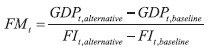 | (1) |
The sizes of implemented shocks are presented in figures 3 and 4, and are obtained by summing up the measures presented in table 2 in their relevant categories according to the ESA methodology, while discarding the categories with the total size of measures of 0.1% of GDP and less due to their marginal effect on GDP. We divided the full year effect of the measures throughout quarters according to the date of their implementation. As structural measures have permanent effects on the level of the budget category, fiscal shocks are applied for each quarter in the consolidation period. We implemented shocks to exogenous fiscal variables in terms of absolute deviations from the baseline scenario (in HRK mn), which allows a direct interpretation of fiscal multipliers in units. However, changes in revenue categories were obtained through shocks to implicit tax/contribution rates.
Revenue-side instruments Table 2 presents fiscal multipliers for different revenue-side instruments used during the EDP. The table shows that, depending on the instrument, the sizes of the multipliers range from -0.3 in the case of personal income tax to 0 for healthcare contributions. These results are mostly in line with model-based estimations of fiscal multipliers presented in Spilimbergo, Schindler and Symansky ( 2009), Gechert and Will ( 2012), and Kilponen et al. ( 2019). These authors report tax multipliers in the range of -0.5 to -0.1, meaning that direct tax multipliers are higher than indirect tax multipliers (also see appendix 4).
Table 2Fiscal multipliers: revenue-side instruments DISPLAY Table
The average indirect tax multiplier in our model stands at -0.1. The negative sign indicates that the increase of indirect taxes leads to a fall of GDP, while the size of the multiplier indicates relatively weak macroeconomic effects of changes in indirect taxes. As figure 6 indicates, the transmission mechanism in this case is based on the effects of indirect taxes on prices, which then affect real disposable income and consumption. However, an empirically based estimate of the pass-through effects of indirect taxes to prices in Croatia, presented in CNB ( 2019) and Buljan ( 2020), indicate that the pass-through is not full and it is estimated to around 0.6. Thus, changes in indirect taxes do not fully translate into changes in prices, which subdues the effect of indirect taxes on real disposable income. The effects of changes in indirect taxes on consumption are additionally mitigated by the fact that only part of the real disposable income is used for consumption. In addition, in economies with a relatively high level of import-dependency, such as Croatia, a notable part of the effects of indirect taxes on consumption (and indirectly on investments) is offset by changes in imports.
The next important fiscal instrument comprises direct taxes. We estimate the average personal income tax multiplier at -0.2, which is quite strong as compared to the effects of indirect taxes, in line with the theoretical and empirical findings. This is because changes in direct taxation directly affect and are fully transmitted to the nominal disposable income. However, the multiplier is still relatively low as changes in disposable income affect consumption only partially. In addition, as in the previous case, changes in imports offset the effects of changes in consumption (appendix 1).
Corporate income tax affects the aggregate demand through the effects on investments, i.e. investment costs. However, corporate income tax presents only a small portion of total investment costs. In addition, investments contain a substantial import component, which means that part of increased investment automatically translates to higher imports (appendix 1). Thus, changes in this tax form do not have pronounced effects on GDP, in line with findings in related literature.
Finally, the average fiscal multiplier for healthcare contributions is -0.1. At first, this result may seem a bit surprising. However, our model captures two effects that act in opposite directions. First, the increase of healthcare contributions increases the costs of investment and leads to a fall in investments, employment and thus in disposable income. On the other hand, the increase of healthcare contributions increases the total compensation of employees in the public sector. As this is one of the key components of government consumption G, which directly enters the GDP equation (7), this effect can offset the fall in private investments and consumption. Nonetheless, a modelling approach that also included the supply-side effects of this measure would yield larger fiscal multipliers, especially in the long run.
Expenditure-side instruments Table 3 presents the fiscal multipliers for these instruments. The table shows that, depending on the instrument, the sizes of the multipliers range from 0.3 in the case of social benefits to 1.3 for public wages. Thus, as expected, fiscal multipliers for expenditure-based measures are in (absolute terms) higher than those of revenueside measures.
These results are also mostly in line with model-based estimations of fiscal multipliers presented in Spilimbergo, Schindler and Symansky ( 2009), Gechert and Will ( 2012), and Kilponen et al. ( 2017). The authors report model-based government consumption multipliers in the range from 0.5 to 0.9 and social benefits multipliers in the range from 0.2 to 0.4. On the other hand, fiscal multipliers of public investment are usually above one (although most estimates are for more closed economies), while in our case the public investment multiplier is below one. Finally, we report the size of the fiscal multiplier of public wages, which is especially interesting as there is almost no model-based literature on public wage multipliers, while other empirical and theoretical results are ambiguous.
Table 3Fiscal multipliers: expenditure-side instruments DISPLAY Table In our model, public sector wages have the largest multiplier, of around 1.3. Such a large multiplier reflects two channels of fiscal policy transmission. First, as previously noted, public sector wages are an important component of government consumption that directly enters the equation (7) for the calculation of GDP. As this component of government consumption does not have an import component it translates to GDP “one-for-one”. Additionally, any increase of (net) public sector wages increases total disposable income and thus stimulates consumption and finally investments, through higher demand for them. The comparison of our results with those of the existing literature is challenging, as to our knowledge there are no many model-based estimates of public wage fiscal multipliers. 16 However, many authors point out that changes in public sector wages can affect wages in the private sector (see Alesina, Favero and Giavazzi, 2019). In our model, we treat wages in these two sectors as independent, which can have a notable effect on the size of the multiplier. Thus, we discuss the relevance of the assumption on the relation between public and private wages in the section on the limitations of our modelling approach.
Unlike public wages, intermediate consumption does contain an import component. 17 Thus, despite the fact that intermediate consumption also directly affects GDP (7), this effect is less than “one for one” as part of the increase of intermediate consumption directly flows to imports. The second-round effects then operate through increased investment demand, which leads to higher investments and employment and thus higher consumption. However, these second-round effects are rather small as government consumption presents a small portion of total investment demand so the size of the multiplier is mostly determined by the firstround effect, i.e. the direct effect on GDP through the national accounting identity. Our estimate of the intermediate government consumption multiplier is 0.6, which is as expected, due to the openness of Croatian economy.
As for subsidies, our results point to a relatively low fiscal multiplier of around 0.1. A low size of the multiplier was expected as subsidies affect the economy only through the effect on investments. However, this effect is not strong. This especially holds true in countries like Croatia, where subsidies are used more as grants and less as investment-promoting instruments, i.e. they are not efficient (World Bank, 2014). Generally, the literature treats subsidies as an unproductive component of government expenditure and OECD positions subsidies at the top of the list of the instruments used in growth-friendly consolidation packages (Cournède, Goujard and Pina, 2013).
The public investment multiplier estimated in our model stands at around 0.7. As in other model-based analyses, the multiplier for this component of government expenditures is higher compared to the intermediate consumption multiplier. However, as previously noted, most papers report public investment multipliers above one, even in open economies. The reason why the multiplier in our model is somewhat low compared to other analyses is that our model includes only the short-run demand-side effects of public investments (appendix 1).
Finally, we estimate the fiscal multiplier for social benefits at around 0.3, which is in line with the findings in model-based literature. Social benefits affect the economy through the effects on disposable income and thus consumption (first-round) and induce an increase of investments through higher investment demand (second-round) (appendix 1). The size of the multiplier is in this case mostly determined by the marginal propensity to consume out of disposable income and by the openness of the economy.
Role of automatic stabilizers In the explanation of transmission mechanisms so far, we consciously neglected the role of automatic stabilizers, due to the brevity of the exposition. However, automatic stabilizers, i.e. the automatic reaction of fiscal variables to changes in economic activity, are an important determinant of the size of fiscal multipliers (Peackok and Shaw, 1976; Batini, Eyraud and Weber, 2014). Every fiscal measure that affects economic activity leads to a feedback effect from economic activity to fiscal variables. For example, as we explained previously, any increase in government consumption will tend to increase investments, employment and consumption, while changes in these macro variables will lead to an increase of corporate income tax, personal income tax and VAT revenues. This raises the tax burden in the economy and alleviates the total effects of the initial fiscal impulse on economic activity. Thus, all fiscal multipliers reported in this paper also capture the role of automatic stabilizers.
5.2 Counterfactual policy analysis
Our analysis so far showed that the EDP fiscal consolidation in Croatia was successful in terms of fiscal outcomes. On the other hand, the reported fiscal multipliers imply that the consolidation measures had detrimental effects on growth throughout the whole consolidation period.
In this sense, our results confirm the Commission’s assessment that implementation of the EDP measures would keep the Croatian economy in recession in 2014 (table 1) and lead to lower growth rates in 2015 and 2016. In the no-policy change scenario the 2014 growth rate was projected to be around 0.5%, while the EDP scenario implied a fall of GDP. In 2015 and 2016 under the EDP scenario, the Commission projected positive growth rates, if around 0.6pp lower than in the no-policy change scenario. This motivated us to take an additional step in our analysis and provide an illustrative counterfactual policy analysis 18 based on an alternative, growth-friendly, fiscal consolidation package. 19
The basic idea behind growth-friendly fiscal consolidations is to design a fiscal consolidation package that ensures improvement of the fiscal balance, while minimizing negative short-term effects on growth (Cournède, Goujard and Pina, 2013). This implementation of consolidation measures could lead to an additional increase in instead of the stabilization of the debt-to-GDP ratio. Thus, ill-conceived design of fiscal consolidation packages can lead to “self-defeating” consolidation episodes. Eyraud and Weber ( 2013) provide a relatively simple framework for the understanding of these contradictory effects of fiscal contractions on public debt dynamics. They explain an “unpleasant fiscal arithmetic” that shows that the debt ratio does not decrease one-for-one with fiscal tightening. The reason for this is that fiscal contraction leads to a fall in economic activity through the fiscal multiplier mechanism. Then, lower economic activity leads to a higher (not lower) share of public debt in GDP for two reasons. First, the fall in GDP decreases the denominator of the debt-to-GDP ratio (“denominator effect”). Second, the fall in GDP also reduces government revenues, which can increase the deficit (“numerator effect”). The total effect of fiscal contraction on public debt dynamics in the short run depends on the size of the fiscal multiplier, the initial level of public debt and the strength of automatic stabilizers (i.e. elasticity of revenues to GDP). These relations can be described by the equation:  | (2) |
The first term on the right side of the equation shows that the implemented consolidation fiscal effort reduces the debt-to-GDP ratio (“direct effect of fiscal consolidation”). However, this effect is mitigated by the above mentioned “denominator effect” (second term on the right side) and the “numerator effect” (third term on the right side). The higher the fiscal multiplier, the stronger are the mitigating effects.
Having this in mind, in the counterfactual analysis we propose a consolidation package that lowers the size of the weighted fiscal multiplier on the expenditure side of the budget. 20 The structure of the consolidation package is presented in table 4, which shows that we only changed the structure of the expenditure-based measures, while keeping the revenue-side measures unchanged. Regarding the size of total fiscal effort, our package is in line with the structural adjustment in the original EDP scenario. There are four main differences in our growth-friendly consolidation package from the EDP consolidation package that was actually implemented.
First, in our view, a growth-friendly consolidation package should keep public investments intact. This view is also supported by the Commission which points out that many EU countries cut investments during the EDP as such measures are politically expedient as compared to cuts in other current expenditure categories. However, the Commission also emphasizes that cuts in public investments have a negative impact on growth and affect debt dynamics (European Commission, 2020). The SGP framework even gives special treatment to public investments in the calculation of the MTO, i.e. allows room for budgetary manoeuvre, in particular taking into account the needs for public investment. 21 Thus in our growth-friendly fiscal consolidation package, policy makers would not rely on cuts in public investments. 22
Table 4Growth-friendly fiscal consolidation package DISPLAY Table
Our model suggests that cuts in public sector wages during recessions can lead to substantial pro-cyclical effects as they yield the largest fiscal multipliers. However, we are aware that the public sector wage bill in Croatia is excessive (e.g. World Bank, 2014) and many relevant authors point to important confidence and credibility effects triggered by cuts in the public sector. As we explained in section 2, cuts in public sector wages signal the commitment of policy makers to the implementation of structural reforms. Thus, our growth-friendly fiscal consolidation package would rely only minimally on cuts in public wages. More precisely, in our counterfactual scenario we propose a package that would include 3% cuts in gross public wages but without additional cuts in holiday and loyalty bonuses.
Third, we already mentioned that subsidies are generally viewed as an unproductive component of government expenditure. Thus, in our counterfactual scenario we propose substantial cuts in subsidies. Rationalization of subsidies was also proposed as a fiscal consolidation measure by the World Bank in the Public Finance Review Croatia in 2014. In addition, Cournède, Goujard and Pina ( 2013) and Kolev and Matthes ( 2013) position subsidies at the top of the list of the instruments used in growth-friendly consolidation packages.
Finally, data on general government expenditures indicate that Croatian authorities disburse notable funds on capital and current transfers. For example, in the period from 2013 to 2016 these expenditures amounted on average to over 10 billion HRK. These expenditures are usually directed to inefficient public-owned enterprises (e.g. invoked guarantees of un-restructured shipyards). In our view, part of these expenditures that would be aimed at restructuring could be transferred to EU funds, while the other part could be rationalized. As these transfers are not recognized as a productive part of government expenditure we would not expect them to yield high multipliers. More precisely, in our model they do not trigger any multiplicative effects on the economy although they do affect fiscal balances.
A growth-friendly consolidation package would yield a lower expenditure-side multiplier (table 5), thus soothing the mitigating effects defined in equation (2). As previously explained, lower fiscal multipliers would thus reduce the probability of self-defeating fiscal consolidation episodes.
Table 5Weighted expenditure-based fiscal multipliers DISPLAY Table
In order to analyse the effects of the proposed growth-friendly fiscal consolidation package we evaluated fiscal and macroeconomic outcomes in the counterfactual scenario and compared it to the EDP baseline scenario. We then calculated the differences between outcomes in the two scenarios and applied these differences to actual data to make the results easier to interpret (figure 7).
Our results indicate that the EDP fiscal consolidation strategy was partially selfdefeating since the unfavourable composition of the fiscal consolidation package led to weaker economic activity and thus to a higher public debt-to-GDP ratio than would have been the case in the alternative scenario, based on the growth-friendly consolidation package. According to the results of the counterfactual scenario, had a more growth-friendly fiscal consolidation package been implemented, recession in Croatia could have ended in 2014. However, it is important to emphasize that in both scenarios public debt-to-GDP ratio increases in the first year of consolidation. This is because in both scenarios interest rates notably exceed GDP growth, thus triggering a snowball effect, while the general government budget records a primary deficit. These two factors were identified as the main drivers of public debt in 2014 (see figure 5). Figure 7Fiscal and macroeconomic outcomes of the EDP and counterfactual scenario DISPLAY Figure
The illustrative counterfactual analysis presented in this section serves only as an illustrative example. Nonetheless, it shows that the design of fiscal consolidation packages can have notable effects on macroeconomic and fiscal outcomes during fiscal consolidation episodes. Thus, in our view, policy makers in Croatia should in the future rely more on this kind of model-based evaluation and take into account the different macroeconomic effects of various fiscal measures.
5.3 Main methodological limitations
Before we move to the conclusions, it is important to explain some of the key limitations of our modelling approach.
As previously noted, the purpose of this model is to provide an analytical framework for the analysis of the short-term macroeconomic effects of fiscal policy. Thus, this model does not include the supply side of the economy and variables such as the potential GDP, the natural rate of unemployment, demographic changes and TFP. These variables are crucial for the long-term analysis but do not play a decisive role in short-term analyses. Of course, we are aware that the exclusion of these factors can have some important effects in the short run as well. For example, the literature shows that public investments have the largest multiplier among all government expenditure components because they stimulate aggregate demand but also increase the overall productive capacity of the economy, through capital accumulation. In addition, standard models of inflation include the output gap or deviation of the unemployment rate from the natural level as important determinants of price developments. Next, changes in direct taxes do not affect only the demand but also the supply side of the economy, through the effects on incentives to work. Our model cannot capture these effects.
However, this does not mean that we have completely neglected the role of some other important supply-side factors in the short run. As we showed in the paper, we recognize that inflation can be affected not only by demand-side factors but also by oil-price shocks and import prices or that decisions on private investments do not depend only on demand for investments but also on the costs (labour costs and corporate tax). In this way, we tried to overcome some of the main shortcomings of purely demand-driven models in the Keynes-Klein tradition (Challen and Hagger, 1983; Wallis and Whitley, 1991).
Another important weakness of our model is that it does not include the monetary authority. From the theoretical and empirical point of view, the most important role that the monetary authority plays in these kinds of analyses is based on its reactions on the money market and the foreign exchange market after the implementation of fiscal measures. If, for example, fiscal expansion leads to a countercyclical increase of the key monetary policy interest rate, the macroeconomic effects of fiscal expansion can be subdued (Ramey, 2011; 2019). As for the reactions on the foreign exchange market, it is well known that fiscal policy is more effective in countries with stabilized exchange rate regimes (Perotti and Lane, 1996) as potential appreciation pressures in times of fiscal expansion are subdued by FX interventions. The reason why we did not include a monetary policy block in our model stems from the specific nature of the monetary policy framework in Croatia which is based on the exchange rate as the key monetary policy anchor. This makes FX interventions a key monetary policy instrument. Thus, in our model we could not include some explicit monetary policy rule, such as the Taylor rule, which is applicable for inflation-targeting countries. Bokan and Ravnik ( 2018) proposed an implicit monetary policy rule for Croatia, based on the reactions of monetary policy to deviation of exchange rate and inflation rate from implicit targets. Although their proposal represents a notable contribution to the literature and covers the effects of monetary policy on exchange rate developments, it does not provide a complete coverage of the effects of FX interventions on money supply and liquidity. In addition, as Bokan et al. ( 2009) and Galac ( 2011) show, the Croatian National Bank relies on many other (regulatory) instruments that can have notable effects on liquidity and money supply in the Croatian economy. Although all the aforementioned factors can have notable effects on the effectiveness of fiscal policy, the development of a model with a monetary block that includes all these factors goes beyond the scope of this paper. Also, in the period from 2014-2016, which is in the focus of our analysis, there were no major changes in monetary policy in Croatia. Thus, in our view, our main conclusions would not be altered even if we explicitly included the monetary policy block in the model.
The next important limitation of the model is a result of our decision to treat exports as an exogenous variable. The effects of fiscal policy on exports can arise from the effects of fiscal policy on nominal exchange rate, consumer prices and producer prices (through labour costs). Thus, in some circumstances, the effects of fiscal policy on exports can hinder the effects of fiscal policy on domestic demand. However, in our view, the decision to treat exports as an exogenous variable can be seen as plausible, if one takes into account several factors. First, the series of exports of goods and services in Croatia in the period of our analysis was dominated by various specific factors, such as exports of ships, tourism revenues, effects of the accession to the EU, etc. The other, more important reason is that exports in Croatia are significantly more sensitive to exogenous changes in foreign demand than to changes in relative prices (Bobić, 2010). In addition, Croatian National Bank data show that the average change of the real effective exchange rate in the period from 2014-2016 stood at around only 1% to 2%. 23 Hence, we do not expect that changes in fiscal policy had a decisive effect on exports developments during the EDP.
Next, we treat public sector and private sector wages independently. However, changes in public sector wages can affect private sector wages and thus induce changes in private sector consumption, investments and employment. Alesina, Favero and Giavazzi ( 2019) state that a reduction in the public sector wage bill has a depressing effect on aggregate demand, but that may be compensated for by the fact that a reduction in public sector wages could translate into lower private sector wages, thus raising profitability and investment. For Croatia, there is some evidence that the public sector leads long-run wage dynamics. Orsini and Ostojić ( 2015) showed that public sector wage in Croatia is independent from wage dynamics in other sectors, while exerting an attraction force on wages in other sectors. This fact can notably affect the estimated size of the fiscal multiplier of public sector wages.
Although theory argues that investments should depend on the level of interest rates on corporate loans, in this paper we did not include this determinant of investments in our investment function. The reason is that in Croatia it is hard to find a statistically significant relationship between interest rates and investments. 24 This was also confirmed in Tica ( 2007), who reviewed the literature on the transmission mechanism of monetary policy in Croatia and concluded that it seems that the IS curve in Croatia is vertical. This can be explained by the fact that only around 25% of total investments are financed by loans 25 and that large companies often use external sources of financing, which additionally breaks the link between domestic interest rates on loans and investments. Although empirically and economically plausible, the decision to exclude interest rates from the investment function has an important drawback. With no interest rates in the model we cannot take into account the relation between the risk premium, mostly determined by developments of public debt, and investments, i.e. we cannot capture the potential “crowding-out” effect. This is important because Kunovac and Pavić ( 2018) found that the risk premium, if increased, will spill over to higher interest rates on loans, especially in the corporate sector. However, with no empirically determined relation between interest rates and investments, the effect of the rise in risk premium on investments could be less pronounced than expected.
Finally, results of all model-based analyses always depend on the main theoretical assumptions and the empirical nature of the model. As we stated before, our model is mostly demand-driven and Keynesian in nature. Thus, our model cannot generate Ricardian reactions of economic agents (e.g. a rise in government consumption raises interest rates, reduces the present value of wealth and thus reduces consumption). In addition, expectations do not play an important role in our model. All these factors can affect the size of calculated fiscal multipliers. As for the empirical nature, we emphasized that our model is not structural, which means that it is subject to Lucas’s critique (Lucas, 1976), like other semi-structural models.
Given all these limitations, we take the results of our analysis with a grain of salt. However, we hope that the analysis provides a solid foundation for future modelbased evaluations of the macroeconomic effects of fiscal policy in Croatia and a framework for understanding of complex fiscal policy transmission mechanisms.
6 Conclusion
Fiscal consolidations are always a subject of intensive public and professional debate. The reason is that, apart from the social dimension of fiscal consolidation programs, the effects of fiscal consolidations on economic activity presented in literature are somewhat ambiguous.
In this paper, we tried to contribute to the understanding of the macroeconomic effects of fiscal consolidations in Croatia, using the EDP episode as a case study. For this purpose, we developed a semi-structural macro-fiscal model of the Croatian economy (MFMC). With its disaggregated fiscal sector, the model offers a deeper insight into the transmission mechanisms of various fiscal instruments on Croatian economy.
The main result of our model-based analysis are disaggregated fiscal multipliers that capture the first-round and second-round effects of the fiscal measures implemented during the EDP. Our estimates of fiscal multipliers for revenue-based (0-0.3) and expenditure-based (0.3-1.3) fiscal instruments are mostly in line with the current literature and characteristics of Croatian economy. Data on disaggregated multipliers can help policy makers in designing the consolidation packages that can deliver the required fiscal effort while minimizing the negative short-term effects on growth.
However, non-complementarity and an ad hoc introduction of fiscal measures, together with a high degree of policy uncertainty during the 2014-2016 EDP episode, weighed down on Croatia’s pursuit of a growth-friendly consolidation strategy. Thus, although it successfully stabilized the public-debt-to-GDP trajectory, Croatia’s fiscal consolidation strategy was growth-detrimental and partially selfdefeating. Our analysis suggests that an alternative choice and timing of fiscal instruments would have shortened the recession in Croatia and improved the overall fiscal outcomes.
As Croatia is preparing to join the euro area in the near future, sustainability of public finances, as one of the key nominal convergence criteria, will be at the top of the economic policy agenda. Thus, we can expect that fiscal policy makers in Croatia will have to engage in a new fiscal consolidation episode in the medium run. In this context, we hope that our results can help policy makers to avoid the policy mistakes made during the EDP.
Appendix
Appendix 1: Model blocks and equations
Aggregate demand
This block defines the behaviour of the main components of aggregate demand. GDP, consumption, private investments and imports are determined endogenously in this block, while we treat exports, government consumption and government investments as exogenous variables. 26 All macro variables are expressed in real terms, 27 which is standard in this type of model.
The consumption function in our model is broadly based on Modigliani’s lifecycle consumption theory. Thus, private consumption depends on disposable income YDt and wealth Wt. Disposable income is defined as the total income (sum of gross wages, government transfers and remittances) minus income taxes and social contributions paid by employees. As there is no publicly available long time series of quarterly data on household financial wealth in Croatia, we approximate it by the deflated stock-exchange index CROBEX. 28 Dt is a dummy variable that takes the value of 1 in the case of some outliers in the data. The long run consumption function is defined as: 29| log(Ct) = C0 + C1log(YtD) + C2log(Wt) + Dt + εtC | (A.1) |
while the short-run equation is then defined as: | dlog(Ct) = c0 + c1dlog(YtD) + c2dlog(Wt) + c3εCt-1 + μct | (A.2) |
The term c3εCt-1 captures the error correction mechanism.
Total real investments are defined as the sum of private investments and government investments.  | (A.3) |
Private investments are the function of investment demand IDt (sum of consumption, exports and government investment) (accelerator effect), foreign direct investment FDIt, costs of production COSTt (defined as the sum of gross private wages and corporate tax per unit of investment) and subsidies in the previous quarter SUBSt-1. Subsidies are included in the model with a lag because we cannot expect this type of government support to companies to be able contemporaneously to increase investment activity. | log(IPt) = I0 + I1 log(IDt) + I2 log(FDIt) + I3(COSTt) + I4 log(SUBSt-1) + εIt | (A.4) |
| dlog(IPt) = i0 + i1dlog (IDt) + i2dlog (FDIt) + i3d (COSTt) + i4dlogg(SUBSt-1) + i5εIt-1 + μIt | (A.5) |
Imports are determined by the import demand ( MDt) in the economy (sum of domestic demand and exports) and terms of trade, which are defined as the ratio of export and import prices. Dt is a dummy variable that takes the value of 1 in case of some outliers in the data:  | (A.6) |
 | (A.7) |
Real gross domestic product based on the expenditure approach can be understood as the total aggregate demand in the economy: 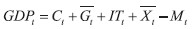 | (A.8) |
On the labour market we define private employment EMPPRIVt and public employment EMPUBt. Private employment is a function of investment activity and private consumption, 30 while public employment is defined exogenously. Dt is a dummy variable that takes the value of 1 in case of some outliers in data: | log(EMPPRIVt) = EMP0 +EMP1log(ITt-1) + EMP2log(Ct-1) + Dt + εtEMP | (A.9) |
| dlog(EMPPRIVt) = emp0 + emp1dlog(ITt-1) + emp2dlog(Ct-1) + emp3εt-1EMP + Dt + μtEMP | (A.10) |
The behaviour of private investment is broadly based on orthodox Keynesian theory where employment is mostly determined by domestic demand (Snowdon and Vane, 2005). However, as there are rigidities on the labour market we expect that components of domestic demand can affect labour market only with a lag.
Total employment is given by the term: 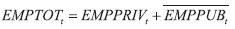 | (A.11) |
Total compensation of employees WTOTALt is then the sum of compensation of employees in the private sector and compensation of employees in the public sector. Compensation of employees is defined as the sum of net wages per employee, income taxes per employee, social contributions for healthcare security per employee and social contributions for pension security per employee multiplied by the number of the employed. All variables are treated exogenously besides private sector employment: 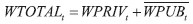 | (A.12) |
The equation that describes the dynamics of prices is broadly based on an open economy version of the Phillips curve. 31 As Croatia has a small open economy, prices are determined by both domestic and external factors (Jovičić and Kunovac, 2017). In addition, when modelling inflation behaviour in Croatia, it is important to consider the “stickiness” of prices (Pufnik and Kunovac, 2013). Having all this in mind, our inflation equation takes the following form: dlog(CPIt) = π0 + π1dlog(CPIt-1) + π2dlog(WTOTALt-1) + π3dlog(MPt) +
π4dlog(OILt) + π5d(IMPL_INDt) + Dt + εtCPI | (A.13) |
The equation shows that quarterly inflation is determined by the quarterly inflation from the previous quarter (sticky prices argument) CPIt-1, changes in total compensation of employees in the previous period WTOTALt-1 that captures the effect of both demand-side and cost-push pressures, changes in import prices MPt, changes in oil prices OILt expressed in Croatian kuna and changes in implicit indirect tax rate ( IMPL_INDt). Dt is a dummy variable that takes the value of 1 in case of some outliers in data.
Fiscal sector One of the main purposes of the model is to estimate the effects of the fiscal consolidation measures implemented and to analyse the transmission mechanisms of fiscal policy. To capture the full effects of various revenue and the expenditure measures on the economy, we have disaggregated the fiscal sector as much as possible. The fiscal categories fully reflect ESA methodology. Key relations among variables in the fiscal block are presented in appendix 5.
We start from the basic identity of the fiscal balance, which is the difference between total general government revenues and expenditures: From here, we disaggregate the total general government revenues, 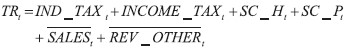 | (A.15) |
where total revenues are the sum of the indirect and income taxes, social contributions for health and pension insurance, government sales and other revenues. Indirect taxes are defined as a product of implicit indirect tax rate and nominal consumption as relevant macroeconomic base:  | (A.16) |
On the other hand, income taxes consist of corporate income tax (CIT) and personal income tax (PIT): | INCOME_TAXt = CITt + PITt | (A.17) |
where, as with indirect tax, corporate income tax is defined as the product of the implicit corporate tax rate and private investment: 32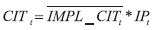 | (A.18) |
On the other hand, personal income tax is divided between private sector and public sector personal income tax to better isolate the effect of income tax changes on private sector and public sector, which is exogenous. Personal income tax is the product of implicit personal tax rates and the compensations of employees: | PITt = PITtPrivate + PITtPublic | (A.19) |
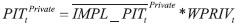 | (A.20) |
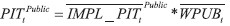 | (A.21) |
Furthermore, social contributions for pension and health insurance are identically divided, and their relevant macroeconomic bases are also compensations of employees: | SC _Pt = SC _PtPrivate + SC _PtPublic | (A.22) |
 | (A.23) |
 | (A.24) |
| SC _Ht = SC _HtPrivate + SC _HtPublic | (A.25) |
| (A.26) |
 | (A.27) |
On the other hand, total general government expenditures are defined as the sum of the government consumption, social benefits (including unemployment benefits), interest, government investment, subsidies, other current and capital transfers: 33 | (A.28) |
Interest expenditure is defined in the public debt section, while unemployment benefits are the function of employment: | dlog(UNEMP _Bt) = UNEMP _B0 + dlog(EMPTOTt) + εtUNEMPB | (A.29) |
Nominal government consumption is defined as the sum of public compensation of wages, social benefits in kind, intermediate consumption, consumption of fixed capital with government sales subtracted:  | (A.30) |
At last, public debt is integrated in the model via traditional decomposition of debt dynamics, where the level of public debt depends on the previous level of public debt and the fiscal balance: | DEBTt = DEBTt-1 + FBt | (A.31) |
Primary fiscal balance is defined as total fiscal balance adjusted for interest expenditures: | FBtprim = TRt – TEt + INTt | (A.32) |
Interest expenditure is annualized and defined as the product of the implicit interest rate and the previous level of debt: | INTtannual = IIRt * DEBTt–4, | (A.33) |
Implicit interest rate is calculated as a ratio of interest expenditures and the level of debt. Their behaviour is modelled as a function of changes in public debt that affect credit rating and borrowing conditions, | dlog (IIRt) = IIR0 + dlog (DEBTt) + εtIIR | (A.34) |
Finally, the decomposition of public debt dynamics is given by the standard formula,  | (A.35) |
Equations (34) and (35) enable us to analyze important feedbacks from macro variables to public debt-to-GDP ratio and feedbacks from debt-to-GDP-ratio to interest rates. These feedbacks can play a crucial role in the success of fiscal consolidations episodes.
The baseline scenario in our analysis is the result of the model estimation for the period from 2003q3 to 2019q4. This scenario includes all fiscal measures implemented during the EDP. All macroeconomic and fiscal variables are obtained from Eurostat, except data on employment, which are based on Croatian Pension Insurance Institute data. The appendix provides a comparison of the simulated baseline scenario and actuals for key macro and fiscal endogenous variables.
Appendix 2: Original and simulated endogenous variables (baseline)
Figure A2.1Endogenous variables – baseline scenario vs. actuals (levels) DISPLAY Figure Figure A2.2Endogenous variables – baseline scenario vs. actuals (growth rates) DISPLAY Figure
Appendix 3: Estimation results – key macro equations
Estimation results – key macro equations
Appendix 4: Fiscal multipliers of different fiscal instruments
Table A4.1Model-based approach DISPLAY Table
Appendix 5: Announced structural measures during the EDP
Table A5.1Announced structural measures during the EDP DISPLAY Table
Appendix 6: More details on the EDP in Croatia
The Recommendation issued in December 2013 required Croatia to correct its excessive deficit by 2016, with an annual improvement in the structural balance of 0.5%, 0.9% and 0.7% of GDP in 2014, 2015 and 2016. The Commission estimated that the mentioned consolidation required Croatia to adopt structural consolidation measures of 2.3% of GDP in 2014 and 1% of GDP in 2015 and 2016 (European Commission, 2013b). It was assessed that these measures would reduce the nominal deficit to below 3% of GDP by 2016 and put the public debt on a sustainable path.
Table A6.1Forecast of macro and fiscal variables under baseline and EDP scenario (December 2013) DISPLAY Table
The Recommendation set a deadline of three months for Croatia to undertake a fiscal effort, i.e. until 30 April 2014. In January 2014, the Council adopted both the Commission’s proposal for a decision on the existence of the excessive deficit and the recommendation on its correction, and officially activated the EDP for Croatia (European Commission, 2014b).
In response to Recommendations of the Council, in March 2014 the Croatian Parliament adopted a supplementary budget of the central government for 2014, which included a package of structural measures of 1.9% of GDP for 2014. As the size of the announced structural measures was below the Commission’s recommendations, additional fiscal measures were adopted in April in the amount of 0.4% of GDP. In the same month, the Government introduced the Convergence Program, which adopted structural measures to correct the excessive deficit in 2015 and 2016, amounting to 1% of GDP in those years.
At the beginning of June 2014, the Commission published an assessment of Croatia’s fiscal effort, where Croatia received a positive assessment of fiscal effort for 2014 and 2015 (European Commission, 2014a). Thus, the nominal target in 2014 was achieved in accordance with the recommendation, while in 2015 it was breached by 0.25% of GDP. The evaluation therefore noted that the 2015 Budget needed to adopt additional structural measures that would enable the achievement of the nominal target in 2015. However, according to the criterion of the “bottomup” analysis, i.e. summarizing structural measures, Croatia met the requirements of the recommendation.
With the expectation that the 2015 Budget would include additional structural adjustment to meet the set targets, the Commission proposed to put the EDP on hold and announced further close monitoring of public finances. Although Croatia struggled to deliver the required structural effort through 2015 (as noticed by the Commission while assessing the Convergence Program for 2015 (European Commission, 2015)), the Procedure stayed in abeyance and no further action by the Commission was pursued.
The EDP timeline When looking at the EDP fiscal consolidation episode in Croatia, we can identify three main policy phases: pre-EDP consolidation phase, main EDP consolidation phase and implementation phase (see figure 1).
1) Pre-EDP consolidation phase This phase started in 2013 and ended with the 2014 Budget revision that anticipated the activation of the EDP for Croatia and already tackled the unsustainable trajectory of Croatia’s public finance. The most significant measures from this period were a public sector wage bill cut in 2013 and other measures implemented with the 2014 Budget, such as pensions cut for the war veterans and a rise of the intermediate VAT rate. The Commission assessed in its December 2013 Report that those measures were not sufficient to correct the excessive deficit.
2) Main EDP consolidation phase In this phase, Croatian authorities introduced the main consolidation package after the official activation of the EDP. The package included the main consolidation measures presented in the 2014 Budget revision and additional measures from April 2014. The consolidation package followed the Commission recommendation with 2.3% of GDP structural measures in 2014 and 1% of GDP in both 2015 and 2016. After the introduction of the package, the Council decided to put the EDP procedure in abeyance. The main measures on the revenue side included an increase of the health contribution, oil and tobacco excises, limitation of CIT tax relief and the introduction of tax on savings, while the expenditure side measures included cuts in investments, intermediate consumption, subsidies and additional cuts of wage bill, through loyalty bonuses.
3) Implementation phase This phase continued throughout 2015 and 2016. During this phase, Croatian authorities made adjustments that led to deviations of the size and type of measures initially proposed by the main EDP consolidation package (see table A5.1 in appendix 5 with all measures listed). As the government dropped some of the measures from the consolidation package (e.g. property tax), it intensified some expenditure cuts such as those in subsidies and investment. Furthermore, consolidation was supported by the expenditure restraint from September 2015 to March 2016 determined by the temporary financing of the Budget and the absence of a government with legislative powers.
Table A6.2Timeline of the EDP consolidation DISPLAY Table
Appendix 7: Disaggregated fiscal sector
Figure A7.1Revenues DISPLAY Figure
Figure A7.2Expenditures DISPLAY Figure
Appendix 8: Detailed description of variables and additional identities
Detailed description of variables and additional identities
Notes
* The article was judged the best paper in the regular category in the annual competition for the Prof. Dr. Marijan Hanžeković Prize for 2020. ** The authors would like to thank the three anonymous referees as well as Jurica Zrnc, Ozana Nadoveza Jelić, Ivan Žilić, Iva Tomić and Ivica Rubil for valuable suggestions and comments. The views expressed in this paper are exclusively those of the authors and do not necessarily reflect those of the Croatian National Bank.
1 IMF in Regional Economic Outlook: Europe October 2020 (p.11) states that: “The extraordinary policy support needs to be anchored by credible consolidation plans to be implemented once the recovery has taken hold.”
2 Fall in GDP reduces the denominator of the ratio but also triggers the mechanism of automatic stabilizers that leads to a fall in revenues and a rise in some categories of expenditures (e.g. unemployment benefits). We explain these mechanisms in more detail in Section 4.
3 Some authors use micro-simulation models to estimate the effects of various fiscal measures on micro level. See for example Urban et al. (2018).
4 These include changes in fiscal variables due to the mechanism of automatic stabilizers and/or counter-cyclical reactions of fiscal policy to business cycle developments.
5 Despite this fact, EDP fiscal consolidation did not attract much attention among academics in Croatia. To our knowledge, the only papers that provide an overview and partial evaluation of this fiscal consolidation episode are Bajo and Galinec (2013), Ujević (2014), Burnać (2017), Deskar-Škrbić and Raos (2018) and Šimović and Deskar-Škrbić (2019). However, these papers have a narrower scope than the present analysis and do not provide empirical assessment of the short-term growth effects of the EDP-based fiscal consolidation.
6 The fiscal multiplier is defined as the ratio of a change in output (∆Y) to an exogenous change in the fiscal variable (∆F).
7 The term "deep structural parameter" was introduced in the 1970s, after Lucas' critic, to distinguish between the derivatives of a behavioral relationship used to define causal effects and the parameters that generate the behavioral relationship (Heckman, 2000).
8 Ministries of finance usually do not have large research departments.
9 The key challenge in this strand of literature lies in the identification of purely exogenous fiscal policy shocks. There are several main approaches to the identification of exogenous fiscal shocks. For detailed overview of different approaches see Ramey (2011, 2019).
10 We provide additional details on the timeline of EDP in Croatia in Appendix 6.
11 However, changes in PIT were not a consolidation measure. According to official wording in the proposal of changes in PIT legislature, this measure was introduced in order to stimulate household consumption and GDP growth.
12 Musgrave (1957) defines macroeconomic stabilization as one of the key functions of public finance, along with redistribution and allocation.
13 In order to assess the overall stability of the model we analyzed impulse responses of various exogenous shocks. Impulse responses in all cases converged and we1 found no evidence of "explosive" impulse responses. These results are available upon request.
14 CPI, implicit rate on public debt and unemployment benefits.
15 Appendix 2 shows the results of the baseline simulation. For more details on estmation results and detailed description of data see Appendix 3 and Appendix 8.
16 Chang et al. (2019) report the public wage multiplier of -0.03 for the US in the NK DSGE model as they calibrate the model in a way that cuts in public wages crowd-in private consumption. However, their model does not take into account the national accounts identity on GDP calculation (eq. 7).
17 Using input-output data for the Croatian economy Mikulić (2019) estimates the import component of total government consumption at around 20%, which is mostly related to intermediate consumption.
18 We are aware of the fact that counterfactual analyses should be based on structural economic models (not subject to Lucas' critique). Hence, counterfactual analyses presented in this paper should be seen an illustrative analytical exercise.
19 IMF applied similar approach in the analysis of the EDP fiscal consolidation episode in Czechia in 2011 (see Klyuev and Snudden, 2011).
20 We concentrate only on the expenditure-based measures as we showed that revenue-based measures yield relatively low fiscal multipliers.
21 Regulation EC 1466/97.
22 However, we are aware that public investments in Croatia are not fully effective as they are often subject of political corruption (Bađun, 2011).
23 REER based on CPI and PPI. Table H11, Croatian National Bank.
24 We tested different specifications of the model and could not obtain statistically significant result with the expected sign in none of specifications.
25 Croatian Bureau of Statistics data. Publication Investments in Croatia.
26 As explained in the subsection on fiscal variables, we treat most of components of government expenditure as exogenous, while government revenues are mostly determined endogenously. This is a standard assumption in this type of analysis. Overbar () ̅ denotes exogenous variables.
27 We only use nominal data on GDP when we need to calculate the share of fiscal variables in GDP. Nominal GDP is calculated as the real GDP multiplied by GDP deflator that is determined by CPI developments.
28 Although some authors also use house prices as a proxy of wealth, in our view consumption in the short run is determined only be liquid form of assets.
29 Equations also include some dummy variables in case of some unexplainable breaks and/or outliers that cannot be explained by economic factors.
30 This equation also contains quadratic trend to improve the fit of the model. More precisely, although investments and consumption adequately describe the dynamics of private employment they cannot capture the size of the amplitude.
31 Of course, as our model does not include the supply-side block that determines the potential output, this equation does not contain output gap. Instead, we use total compensation to employees as a measure of demand-side pressures. However, this variable also captures some cost-push pressures as rising nominal wages can motivate firms to increase prices.
32 Investments serve as a proxy for gross operating surplus of corporations, which is commonly used as a macro base for corporate income tax. However, this variable is not available for Croatia on a quarterly level.
33 Consumption of fixed capital is subtracted, while government sales are added to annul the terms in government consumption identity.
* The article was judged the best paper in the regular category in the annual competition for the Prof. Dr. Marijan Hanžeković Prize for 2020. ** The authors would like to thank the three anonymous referees as well as Jurica Zrnc, Ozana Nadoveza Jelić, Ivan Žilić, Iva Tomić and Ivica Rubil for valuable suggestions and comments. The views expressed in this paper are exclusively those of the authors and do not necessarily reflect those of the Croatian National Bank.
1 IMF in Regional Economic Outlook: Europe October 2020 (p.11) states that: “The extraordinary policy support needs to be anchored by credible consolidation plans to be implemented once the recovery has taken hold.”
2 Fall in GDP reduces the denominator of the ratio but also triggers the mechanism of automatic stabilizers that leads to a fall in revenues and a rise in some categories of expenditures (e.g. unemployment benefits). We explain these mechanisms in more detail in Section 4.
3 Some authors use micro-simulation models to estimate the effects of various fiscal measures on micro level. See for example Urban et al. ( 2018).
4 These include changes in fiscal variables due to the mechanism of automatic stabilizers and/or counter-cyclical reactions of fiscal policy to business cycle developments.
5 Despite this fact, EDP fiscal consolidation did not attract much attention among academics in Croatia. To our knowledge, the only papers that provide an overview and partial evaluation of this fiscal consolidation episode are Bajo and Galinec ( 2013), Ujević ( 2014), Burnać ( 2017), Deskar-Škrbić and Raos ( 2018) and Šimović and Deskar-Škrbić ( 2019). However, these papers have a narrower scope than the present analysis and do not provide empirical assessment of the short-term growth effects of the EDP-based fiscal consolidation.
6 The fiscal multiplier is defined as the ratio of a change in output (∆Y) to an exogenous change in the fiscal variable (∆F).
7 The term "deep structural parameter" was introduced in the 1970s, after Lucas' critic, to distinguish between the derivatives of a behavioral relationship used to define causal effects and the parameters that generate the behavioral relationship (Heckman, 2000).
8 Ministries of finance usually do not have large research departments.
9 The key challenge in this strand of literature lies in the identification of purely exogenous fiscal policy shocks. There are several main approaches to the identification of exogenous fiscal shocks. For detailed overview of different approaches see Ramey ( 2011, 2019).
10 We provide additional details on the timeline of EDP in Croatia in Appendix 6.
11 However, changes in PIT were not a consolidation measure. According to official wording in the proposal of changes in PIT legislature, this measure was introduced in order to stimulate household consumption and GDP growth.
12 Musgrave (1957) defines macroeconomic stabilization as one of the key functions of public finance, along with redistribution and allocation.
13 In order to assess the overall stability of the model we analyzed impulse responses of various exogenous shocks. Impulse responses in all cases converged and we1 found no evidence of "explosive" impulse responses. These results are available upon request.
14 CPI, implicit rate on public debt and unemployment benefits.
15 Appendix 2 shows the results of the baseline simulation. For more details on estmation results and detailed description of data see Appendix 3 and Appendix 8.
16 Chang et al. ( 2019) report the public wage multiplier of -0.03 for the US in the NK DSGE model as they calibrate the model in a way that cuts in public wages crowd-in private consumption. However, their model does not take into account the national accounts identity on GDP calculation (eq. 7).
17 Using input-output data for the Croatian economy Mikulić ( 2019) estimates the import component of total government consumption at around 20%, which is mostly related to intermediate consumption.
18 We are aware of the fact that counterfactual analyses should be based on structural economic models (not subject to Lucas' critique). Hence, counterfactual analyses presented in this paper should be seen an illustrative analytical exercise.
19 IMF applied similar approach in the analysis of the EDP fiscal consolidation episode in Czechia in 2011 (see Klyuev and Snudden, 2011).
20 We concentrate only on the expenditure-based measures as we showed that revenue-based measures yield relatively low fiscal multipliers.
21 Regulation EC 1466/97.
22 However, we are aware that public investments in Croatia are not fully effective as they are often subject of political corruption (Bađun, 2011).
23 REER based on CPI and PPI. Table H11, Croatian National Bank.
24 We tested different specifications of the model and could not obtain statistically significant result with the expected sign in none of specifications.
25 Croatian Bureau of Statistics data. Publication Investments in Croatia.
26 As explained in the subsection on fiscal variables, we treat most of components of government expenditure as exogenous, while government revenues are mostly determined endogenously. This is a standard assumption in this type of analysis. Overbar () ̅ denotes exogenous variables.
27 We only use nominal data on GDP when we need to calculate the share of fiscal variables in GDP. Nominal GDP is calculated as the real GDP multiplied by GDP deflator that is determined by CPI developments.
28 Although some authors also use house prices as a proxy of wealth, in our view consumption in the short run is determined only be liquid form of assets.
29 Equations also include some dummy variables in case of some unexplainable breaks and/or outliers that cannot be explained by economic factors.
30 This equation also contains quadratic trend to improve the fit of the model. More precisely, although investments and consumption adequately describe the dynamics of private employment they cannot capture the size of the amplitude.
31 Of course, as our model does not include the supply-side block that determines the potential output, this equation does not contain output gap. Instead, we use total compensation to employees as a measure of demand-side pressures. However, this variable also captures some cost-push pressures as rising nominal wages can motivate firms to increase prices.
32 Investments serve as a proxy for gross operating surplus of corporations, which is commonly used as a macro base for corporate income tax. However, this variable is not available for Croatia on a quarterly level.
33 Consumption of fixed capital is subtracted, while government sales are added to annul the terms in government consumption identity.
Disclosure statement
No potential conflict of interest was reported by the authors.
References
Alesina, A. [et al.], 2017. The effects of fiscal consolidations: Theory and evidence. NBER Working Paper, No. 23385 [ CrossRef]
Alesina, A. and Ardagna, S., 2010. Large changes in fiscal policy: taxes versus spending. Tax policy and the economy, 24(1), pp. 35-68 [ CrossRef]
Alesina, A. and Perotti, R., 1995. Fiscal expansions and adjustments in OECD countries. Economic policy, 10(21), pp. 205-248. [ CrossRef]
Alesina, A. and Perotti, R., 1997. Fiscal adjustments in OECD countries: composition and macroeconomic effects. Staff Papers, 44(2), pp. 210-248 [ CrossRef]
Alesina, A., Favero, C. and Giavazzi, F., 2019. Austerity: When it Works and when it Doesn't. Princeton: Princeton University Press [ CrossRef]
Bađun, M., 2011. Odnos političke korupcije i javnih investicija–slučaj Hrvatske. Društvena istraživanja-Časopis za opća društvena pitanja, 20(112), pp. 295-316 [ CrossRef]
Baghli, M. [et al.], 2004. Model for analysing and forecasting short term developments. Banque de France Working Paper, No. 106 [ CrossRef]
Bagliano, F. C. and Favero, C. A., 1998. Measuring monetary policy with VAR models: An evaluation. European Economic Review, 42(6), pp. 1069-1112 [ CrossRef]
Bajo, A. and Galinec, D., 2013. Ten facts about the Excessive Deficit Procedure. Newsletter: an occasional publication of the Institute of Public Finance, 15(80) [ CrossRef]
Barrios, S., Langedijk, S. and Pench, L., 2010. EU fiscal consolidation after the financial crisis: Lessons from past experiences. Bank of Italy Occasional Paper, No. 418 [ CrossRef]
Batini, N., Eyraud, L. and Weber, A., 2014. A simple method to compute fiscal multipliers. IMF Working paper, WP 14/93 [ CrossRef]
Baumgartner, J., Breuss, F. and Kaniovski, S., 2004. WIFO-Macromod. An Econometric Model of the Austrian Economy. WIFO Working Paper, No. 241.
Benkovskis, K. and Stikuts, D., 2006. Latvia's macroeconomic model. National Bank of Latvia Working Paper, No. 2006/02.
Bobić, V., 2010. Dohodovna i cjenovna elastičnost hrvatske robne razmjene–analiza panel-podataka. HNB Istraživanja, I-29.
Bokan, N. and Ravnik, R., 2018. Quarterly Projection Model for Croatia. CNB Surveys, S-34.
Boussard, J., de Castro F. and Salto, M., 2013. Fiscal Multipliers and Public Debt Dynamics in Consolidations. In: L. Paganetto L., ed. Public Debt, Global Governance and Economic Dynamism. Milano: Springer [ CrossRef]
Burns, A. [et al.], 2019. The World Bank Macro-Fiscal Model Technical Description. Policy Research Working Paper, No. 8965 [ CrossRef]
Challen, D. W. and Hagger, A. J., 1983. Econometric Systems: Construction, Validation and Applications. Macmillan International Higher Education.
Challen, D. W., 1983. Econometric Systems: Construction, Validation and Applications. Macmillan International Higher Education.
Chang, J. J. [et al.], 2019. Fiscal Consolidation and Public Wages. IMF Working Paper, No. 19/125 [ CrossRef]
Cortuk, O., 2013. A disaggregated approach to the determination of government spending multipliers. Journal of Economic Policy Reform, 16(1), pp. 31-45 [ CrossRef]
Cournède, B., Goujard, A. and Pina, Á., 2014. Reconciling fiscal consolidation with growth and equity. OECD Journal: Economic Studies, (1), pp. 7-89 [ CrossRef]
Daníelsson, Á. [et al.], 2006. A Quarterly Macroeconomic Model of the Icelandic Economy. Central Bank of Iceland, Working paper, No. 32 [ CrossRef]
Deskar-Škrbić, M. and Raos, V., 2018. The Type of Fiscal Policy and Political Economy of Fiscal Consolidation in Croatia in the Post-Crisis Period. In: Tax Policy and Fiscal Consolidation in Croatia: project = Porezna politika i fiskalna konsolidacija u Hrvatskoj: projekt. Rijeka: Faculty of Economics.
Deskar-Škrbić, M. and Šimović, H., 2017. The effectiveness of fiscal spending in Croatia, Slovenia and Serbia: the role of trade openness and public debt level. Post-communist economies, 29(3), pp. 336-358 [ CrossRef]
Deskar-Škrbić, M., 2018. Dynamic effects of fiscal policy in Croatia: confronting New-Keynesian SOE theory with empirics. Zbornik radova Ekonomskog fakulteta u Rijeci: časopis za ekonomsku teoriju i praksu, 36(1), pp. 83-102 [ CrossRef]
Escolano, M. J. [et al.], 2014. How much is a lot? Historical evidence on the size of fiscal adjustments. IMF Working Paper, No. 179 [ CrossRef]
European Commission, 2013a. Staff Working Document, Analysis by the Commission services of the budgetary situation in Croatia. Bruxelles: European Commission.
European Commission, 2013b. Recommendation for a Council Recommendation with a view to bringing an end to the situation of an excessive government deficit in Croatia, COM/2013/0914. Bruxelles: European Commission.
European Commission, 2014a. Assessment of action taken by POLAND in response to the Council Recommendation of 10 December 2013 and by CROATIA in response to the Council Recommendation of 28 January 2014 with a view to bringing an end to the situation of excessive government deficit, COM/2014/0431. Bruxelles: European Commission.
European Commisssion, 2014b. Council Decision of 28 January 2014 on the existence of an excessive deficit in Croatia, 2014/56/EU. Bruxelles: European Commission.
European Commission, 2015. Assessment of the 2015 Convergence Programme for Croatia SWD/2013/0523. Bruxelles: European Commission.
Eyraud, L. and Weber, A., 2013. The challenge of debt reduction during fiscal consolidation. IMF Working Paper, No. 179 [ CrossRef]
Galac, T., 2011. Središnja banka kao krizni menadžer u Hrvatskoj-analiza hipotetičnih scenarija. Zagreb: Hrvatska Narodna Banka.
Gechert, S. 2015. What fiscal policy is most effective? A meta-regression analysis. Oxford Economic Papers, 67(3), pp. 553-580 [ CrossRef]
Grdović Gnip, A., 2014. The power of fiscal multipliers in Croatia. Financial theory and practice, 38(2), pp. 173-219 [ CrossRef]
Grdović Gnip, A., 2015. Empirical assessment of stabilization effects of fiscal policy in Croatia. Romanian Journal of Economic Forecasting, 18(1), pp. 47-69.
Grech, A. G. [et al.], 2013. A structural macro-econometric model of the Maltese economy. MPRA Paper, No. 46128.
Gros, D. and Maurer, R., 2012. Can austerity be self-defeating?. Intereconomics, 47(3), pp. 175-184 [ CrossRef]
Guichard, S. [et al.], 2007. What Affects Fiscal Consolidation?–Some Evidence from OECD Countries [ CrossRef]
Gόrnicka, L. [et al.], 2018. Learning about fiscal multipliers during the European sovereign debt crisis: evidence from a quasi-natural experiment. ECB Working Paper Series, No. 2154 [ CrossRef]
Heckman, J. J., 2000. Causal parameters and policy analysis in economics: A twentieth century retrospective. The Quarterly Journal of Economics, 115(1), pp. 45-97 [ CrossRef]
Jovičić, G. and Kunovac, D., 2017. What is Driving Inflation and GDP in a Small European Economy: The Case of Croatia. CNB Working Paper, No. W-49.
Jurković, P., 2002. Javne financije. Zagreb: Masmedia.
Kluyev, V. and Snudden, S., 2011. Effects of Fiscal Consolidation in the Czech Republic. IMF Working Paper, No. 11/65 [ CrossRef]
Kolev, G. and Matthes, J., 2013. Smart fiscal consolidation: a strategy for achieving sustainable public finances and growth. European View, 12(2) [ CrossRef]
Kunovac, D. and Pavić, N., 2018. Može li uvođenje eura u Hrvatskoj sniziti trošak zaduživanja? Privredna kretanja i ekonomska politika, 27(142), pp. 71-94 [ CrossRef]
Lucas, R. E., 1976. Econometric policy evaluation: A critique. Carnegie-Rochester conference series on public policy, 1(1), pp. 19-46 [ CrossRef]
Mikulić, D., 2019. Osnove input-output analize s primjenom na hrvatsko gospodarstvo. Zagreb: Ekonomski institut Zagreb.
Molnar, M., 2013. Fiscal consolidation. OECD Journal: Economic Studies, 1, pp. 123-149 [ CrossRef]
Muir, D. and Weber, A. 2013. Fiscal multipliers in Bulgaria: Low but still relevant. IMF Working Paper Series, No. 13-49 [ CrossRef]
Musgrave, R. A. and Musgrave, P. B., 1973. Public finance in theory and practice. New York: Springer Publishing.
Nadoveza, O., Sekur, T. and Beg, M., 2016. General equilibrium effects of lower labor tax burden in Croatia. Zagreb International Review of Economics & Business, 19, pp. 1-13 [ CrossRef]
Orsini, K. and Ostojić, V., 2015. Wage Dinamics in Croatia: Leaders and Followers. Economic Brief, No. 3 [ CrossRef]
Peacock, A. T. and Shaw, G. K., 1976. The economic theory of fiscal policy. London: Allen & Unwin.
Perotti, R. and Lane, P. R., 1996. Profitability, fiscal policy and exchange rate regimes. EPR Discussion Paper Series, No. 144.
Pufnik, A. and Kunovac, M., 2015. Obilježja tržišta rada i određivanja plaća u Hrvatskoj: rezultati Ankete poduzeća. HNB Pregled, No. P-27.
Ramey, V. A., 2011. Can government purchases stimulate the economy? Journal of Economic Literature, 49(3), pp. 673-85 [ CrossRef]
Ramey, V. A., 2019. Ten years after the financial crisis: What have we learned from the renaissance in fiscal research? Journal of Economic Perspectives, 33(2), pp. 89-114 [ CrossRef]
Šimović H. and Deskar-Škrbić M., 2019. Fiscal Policy and European Semester in Croatia: Why Should We Focus on Public Debt? In: Z. Petak and K. Kotarski, eds. Policy-Making at the European Periphery. New Perspectives on South-East Europe. Cham: Palgrave Macmillan [ CrossRef]
Šimović, H. and Deskar-Škrbić, M., 2013. Dynamic effects of fiscal policy and fiscal multipliers in Croatia. Zbornik radova Ekonomskog fakulteta u Rijeci: časopis za ekonomsku teoriju i praksu, 31(1), pp. 55-78 [ CrossRef]
Snowdon, B. and Vane, H. R., 2005. Modern macroeconomics: its origins, development and current state. London: Edward Elgar Publishing.
Snudden, S. and Klyuev, M. V. 2011. Effects of fiscal consolidation in the Czech Republic. IMF Working Paper Series, No. 11-65 [ CrossRef]
Ujević, T., 2014. State Budget Revision for 2014–An Attempt to Fulfill the “EDP” Criteria. Privredna kretanja i ekonomska politika, 23(134), pp. 71-90.
Urban, I. [et al.], 2018. Primjena mikrosimulacijskih modela u analizi poreza i socijalnih naknada u Hrvatskoj: rezultati projekta. Institut za javne financije.
Von Hagen, J., Hallett, A. H. and Strauch, R., 2002. Budgetary consolidation in Europe: quality, economic conditions, and persistence. Journal of the Japanese and International Economies, 16(4), pp. 512-535 [ CrossRef]
Wallis, K. F. and Whitley, J. D., 1991. Large-scale econometric models of national economies. The Scandinavian Journal of Economics, pp. 283-314 [ CrossRef]
Zubairy, S. 2014. On fiscal multipliers: Estimates from a medium scale DSGE model. International Economic Review, 55(1), 169-195 [ CrossRef]
|


