|
|
|
Abstract
This paper estimates Laffer curves for personal income tax, corporate income tax,
and value-added tax across OECD countries. While the Laffer curve is widely used
for assessing the revenue effects of taxation, existing empirical estimates typically
rely on restrictive functional forms and are vulnerable to misspecification, when the
true relationship between tax rates and revenues is unknown. In response to this
limitation, this paper develops a model that allows data-driven flexibility and
enforces the defining properties of the Laffer curve. The parameters governing the
curvature and turning points of the curve depend on a rich set of structural and
institutional characteristics while LASSO regularisation mitigates overfitting. The
results reveal substantial cross-country heterogeneity in revenue-maximising tax
rates among OECD countries and suggest there is limited scope for further revenue
mobilisation through higher income tax rates in several countries, while highlighting
a comparatively greater fiscal space in consumption taxation.
Keywords: optimal taxation; Laffer curve; macroeconomic modelling; LASSO
JEL: H21, C51, C54
1 Introduction
Rising fiscal pressures associated with population ageing, climate mitigation and adaptation, defence spending, and digital investment have renewed policy interest in understanding how changes in tax rates affect public revenue. In this context, the Laffer curve provides a unifying framework to analyse the trade-off between statutory tax rates and the responsiveness of tax bases. While higher tax rates mechanically increase revenues, they may also trigger behavioural, compositional, administrative, and macroeconomic responses that will erode the tax base and ultimately reduce revenue. Identifying the shape of the Laffer curve and the location of its turning point therefore remains central to the design of sustainable and efficient tax systems.
Despite a substantial empirical literature, most reduced-form estimates of the Laffer curve rely on restrictive functional forms – typically quadratic, polynomial, or loglinear specifications – and concentrate on identifying revenue-maximising tax rates in the neighbourhood of observed policy settings. These approaches often neglect key theoretical properties of the Laffer relationship – most notably the requirement that revenues approach zero at tax rates of 0% and 100% – and may suffer from misspecification bias when extrapolated beyond the observed data range.
The true functional relationship between tax rates and aggregate revenues is inherently non-linear and difficult to specify ex ante, particularly in cross-country settings characterised by heterogeneity in economic structures, institutional frameworks, and tax systems. The present paper contributes to the empirical literature by proposing a flexible model, grounded in the constant elasticity model of the taxable income literature, that incorporates the core theoretical properties of the Laffer curve while allowing for a broad range of shapes reflecting country heterogeneity. Rather than unduly restricting the model, these constraints incorporate prior economic structure into the estimation, thereby improving statistical identification, excluding economically implausible functional forms, and enhancing the credibility of out-of-sample extrapolation beyond the observed tax rates range.
The shape of the Laffer curve is modelled as a function of a rich set of structural, institutional, and macroeconomic characteristics. The specification improves estimation precision by pooling information across countries and over time. The model is estimated using a LASSO technique, whose regularisation properties reduce the risk of overfitting, improve out-of-sample predictive performance, and mitigate multicollinearity among structural covariates.
The model is applied to personal income tax (PIT), corporate income tax (CIT), and value-added tax (VAT) data for a panel of OECD countries from 2000 onwards. The analysis yields estimates of revenue-maximising tax rates and highlights substantial heterogeneity across countries, reflecting differences in economic structure, institutions, and tax design. By integrating regularisation techniques into a theoretically grounded Laffer curve framework, this paper advances the empirical literature and provides policy-relevant insights into the scope and limits of revenue mobilisation through tax rate changes.
The remainder of the paper is organised as follows. Section 2 reviews the related literature. Section 3 describes the data. Section 4 presents the model; section 5 presents the estimation strategy. Section 6 discusses the empirical results, and section 7 concludes.
2 Literature review
The empirical estimation of the Laffer curve has produced a substantial body of reduced-form studies that seek to characterise the macroeconomic effects of changes in tax rates on tax revenues, often applying polynomial, hyperbolic, or log-linear functional forms to explore the relationship between average tax rates and tax revenues. Hsing ( 1996) estimated four alternative specifications of the US Laffer curve and found a peak tax rate near 33%. Heijman and van Ophem (2005) applied a quadratic optimisation model to estimate country-specific optimal tax rates for 12 OECD countries, while Liapis et al. (2020) compared multiple functional forms for average personal income tax (PIT) and corporate income tax (CIT) rates in the EU and concluded that quadratic models offer the best fit. Other studies focused on consumption taxes. Matthews (2003) and de Oliveira and Costa (2015) estimated value added tax (VAT), Laffer curves and confirmed a hump-shaped relationship, with peak rates between 20% and 25%. Akgun, Bartolini, and Cournède (2017) extended this approach to a broader set of consumption taxes across OECD countries and found that VAT revenues tend to peak around 19%. Ferreira‐Lopes, Martins, and Espanhol (2019) used implicit tax rates and concluded that several countries operate well below their potential revenue levels. Liapis et al. (2020) and Agersnap and Zidar (2020) applied this methodology to capital taxation, showing that capital mobility in open economies constrains the achievable revenue-maximising rate. 1996) estimated four alternative specifications of the US Laffer curve and found a peak tax rate near 33%. Heijman and van Ophem (2005) applied a quadratic optimisation model to estimate country-specific optimal tax rates for 12 OECD countries, while Liapis et al. (2020) compared multiple functional forms for average personal income tax (PIT) and corporate income tax (CIT) rates in the EU and concluded that quadratic models offer the best fit. Other studies focused on consumption taxes. Matthews (2003) and de Oliveira and Costa (2015) estimated value added tax (VAT), Laffer curves and confirmed a hump-shaped relationship, with peak rates between 20% and 25%. Akgun, Bartolini, and Cournède (2017) extended this approach to a broader set of consumption taxes across OECD countries and found that VAT revenues tend to peak around 19%. Ferreira‐Lopes, Martins, and Espanhol (2019) used implicit tax rates and concluded that several countries operate well below their potential revenue levels. Liapis et al. (2020) and Agersnap and Zidar (2020) applied this methodology to capital taxation, showing that capital mobility in open economies constrains the achievable revenue-maximising rate.
Much of the empirical literature has remained narrowly focused on estimating this optimal point and fitting a polynomial or similar smooth function in its vicinity. This emphasis on local approximation often led to neglect of the key theoretical restrictions of the Laffer curve, such as revenue approaching zero at 0% and 100% tax rates, the increase in revenue away from these endpoints, and the requirement that revenue-to-GDP ratios cannot exceed the corresponding tax rate. Traditional reduced-form specifications assume functional forms – typically quadratic, cubic, or other low-order polynomials – that do not guarantee consistency with the theoretical curvature of the Laffer relationship (figure 1). The resulting misspecification bias may lead to implausible marginal effects or optimal points.
Figure 1Common used function forms for the Laffer curve DISPLAY Figure
The present paper proposes a reduced-form model inspired by the underlying intuition of the elasticity of taxable income (ETI) framework originally developed using microdata. Early studies by Lindsey ( 1987) and Feldstein ( 1995 ) showed that reductions in marginal tax rates led to substantial increases in reported income, especially among top earners, implying that high-income individuals exhibit large behavioural responses. Building on these findings, Saez ( 2001) developed a theoretical formula linking optimal top marginal tax rates to ETI.
The present paper builds on the elasticity-based intuition underlying much of the empirical Laffer curve literature, while adapting it to the explicit objective of modelling aggregate tax revenue as a share of GDP. To this end, the proposed functional form departs from approaches that focus on behavioural responses to marginal tax rates and instead models the aggregate relationship between average tax rates and total revenues. This modelling choice is also consistent with the practice adopted in general equilibrium approaches that analyse the revenue effects of taxation at the macroeconomic level (see, for example, Mankiw and Weinzierl, 2006; Agell and Persson, 2001; Tsuchiya, 2016; Sanz-Sanz, 2016; and Holter, Krueger and Stepanchuk, 2019). When the object of interest is total revenue, the relevant elasticity is not a marginal elasticity defined at a specific income threshold, but an aggregate elasticity that combines behavioural responses, compositional effects across taxpayers, administrative features of the tax system, and broader macroeconomic adjustments. This distinction is particularly important in the context of personal income tax (PIT) and value added tax (VAT) systems, which feature multiple schedules and multiple statutory or effective rates. In such settings, the use of a single marginal tax rate – common in parts of the empirical literature – is not well suited to capture the effective tax burden faced by the economy as a whole. Estimating aggregate revenue effects instead requires a synthetic measure of average taxation that reflects the diversity of tax rates and taxpayer characteristics. Accordingly, for PIT in the present paper, the simple mean of the average tax wedges for eight representative household types that reflect different income levels and family compositions from the OECD Tax Database was used. Similarly, for VAT the simple mean of the standard, reduced, and higher rates was used. Although simplified, these synthetic indicators provide a parsimonious measure capturing the structural relationship between several tax policy instruments and aggregate revenue.
The model proposed in this paper provides a flexible yet disciplined model that incorporates these theoretical properties while allowing the parameters of the curve to depend on structural economic variables. This improves robustness to misspecification and allows for cross-country heterogeneity in a way that traditional functional forms cannot. The use of a LASSO estimator provides a regularisation mechanism, thus reducing the risk of overfitting.
While the application of LASSO-type regularisation to non-linear econometric models is well established in the broader economics and econometrics literature, to the best of the author’s knowledge, no existing study has applied machine learning techniques to the empirical estimation of the Laffer curve. This gap is notable, as the Laffer relationship is characterised by strong non-linearities and binding theoretical constraints, while its empirical functional form remains uncertain.
3 The data
3.1 Dependent variables
The empirical analysis is conducted on an unbalanced panel of 26 OECD countries covering the period from 2000-21. The resulting sample comprises a total of 529 country-year observations, reflecting heterogeneous temporal coverage rather than deliberate sample selection. Following the methodology in Bloch et al. (2016), the following three public revenue aggregates were chosen: personal income taxes, corporate income taxes revenue, and consumption taxes revenue. To assure comparability among countries the three aggregates were expressed as a share of GDP. A summary description of the three revenue aggregates is shown in table 1.
Table 1Summary table of the dependent variables DISPLAY Table
3.2 Tax rates
For the estimation of the Laffer curve the choice of the taxation rate of reference is capital for the analysis. Generally, tax systems have a variety of tax rates, and a synthetic indicator is necessary for both the parametric and the non-parametric approach.
In the case of personal income tax, the tax rates may vary based on family composition, income, and region or state of residence. Moreover, due to the progressivity of the taxation systems, taxpayers’ incomes are subject to increasing marginal tax rates, according to the income brackets. In the present work, the average tax wedge was chosen from the OECD Tax database 1, in agreement with the reasoning that it is the average tax rate that determines the total tax revenue. This indicator corresponds to the ratio between the amount of taxes paid by the taxpayers and the corresponding total labour cost for the employer, measured in percentage of labour cost. The present work uses a simple mean of the average tax wedges of the following household types: (1) a single person earning 67% of the average wage; (2) a single person earning the average wage; (3) a single person earning 167% of the average wage; (4) a single person with 2 children earning 67% of the average wage; (5) a couple without children earning 100% and 67% of the average wage; (6) a couple with 2 children earning 100% and 67% of the average wage; (7) a couple with 2 children both earning the average wage; and (8) a one-earner married couple with two children earning the average wage.
For corporate income tax, the combined corporate income tax rate from the OECD Tax database was used, which combines central and sub-central (statutory) corporate income tax rates.
For VAT some authors, like Matthews ( 2003) and Akgun, Bartolini and Cournède ( 2017) used the standard VAT rate because most of the goods are taxed at the standard rate and, for the available data, the correlation between the standard rate of VAT and the effective tax rate is high. For the present work, however a simple mean of the standard, reduced, and higher VAT rates was used from the OECD Tax database. The correlation between this indicator and the standard VAT rate is around 89% and in addiction it captures the balance between reduced and higher VAT rates.
Table 2Summary table of the tax rates DISPLAY Table
3.3 Independent variables
The set of dependent variables includes a set of indicators of quality of the institutions, of economic activity composition, and demography. The quality of institutions such as government effectiveness, control of corruption, regulatory quality, and rule of law, can improve competition among economic actors, increase the cost of tax avoidance and evasion, and the compliance of taxpayers, affecting in this way the scale effect, the revenue maximizing tax rate and the tax base effect. Moreover, the quality of institutions affects competition, which may affect the curvature of the Laffercurve2.The economic activity composition variables such as the decomposition of the GDP using the expenditure and the output approaches could capture the differences in the economic structures of the countries that may affect the structure of the Laffer curve. Some sectors, for example, may have a stronger presence of informality or unregistered activities and therefore be more likely to evade taxation 3; a country whose GDP is mostly driven by labour intensive sectors may offer less possibility for the evasion or avoidance of personal income taxation; an economy with a strong presence of capital intensive sectors may show strong tax base effects due to an increase in the corporate income tax rate 4; an economy with strong internal consumption may show smaller tax base effects due to an increase in the VAT rate but its GDP may be affected more. The demographic composition of a country can affect the shape of the Laffer curve due to age and gender wage gaps 5. Inflation can alter the tax burden through collection lags, absence of indexation, deductibility of expenditures, interest payments on debt 6. The progressivity indicator of the personal income tax is a measure of the dispersion of the marginal tax rates. It is computed as 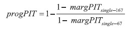 | (1) |
Higher progressivity of taxation is generally associated with lower tax revenues. 7
To reduce the omitted variable bias, the set of dependent variables also includes a set of country fixed effects, which capture the effect of non-observable countryspecific characteristics that do not vary substantially over the sample period.
Table 3Summary table of the independent variables DISPLAY Table
4 The model
The parametric model proposed in this paper is inspired by the elasticity-based framework first introduced by Lindsey (1987) and later formalised by Saez (2001) and Diamond and Saez (2011) to derive optimal tax rates. In their approach, the elasticity of taxable income is used to identify revenue-maximising and welfare maximising tax rates, particularly for high-income earners. The proposed model Laffer curve is derived from the ETI approach and adapted to express revenues as a share of GDP instead of local currency units, as in most of the empirical cross-country literature8: | (2) |
where Tc,i,t represents revenue item i, as a percentage of GDP.
To generate a subset of curves that accurately reflect the Laffer curve, the following parameter restrictions were imposed: α ∈ [0,1], δ ≥ 1, β > 0.
Under these restrictions the proposed model has the following properties: - Tax revenue remains zero when the tax rate is either 0% or 100%.
Τ (τ c,i,t = 0%) = T (τ c,i,t = 100%) = 0
- The curve reaches its maximum at
 with maximum revenue as a share of GDP given by T(τ*) = α ⋅ τc,i,t. with maximum revenue as a share of GDP given by T(τ*) = α ⋅ τc,i,t. - At any point on the curve, the estimated tax-to-GDP ratio does not exceed the corresponding average tax rate

 | (3) |
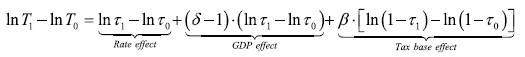
- The tax rate effect measures the increase in tax revenues due a rise in the tax rate, assuming the tax base and the economy remains unaffected. It depends solely on the initial tax rate, and it is independent of other parameters.
- The tax-base effect captures the responsiveness of the tax base to changes in the tax rate, reflecting tax avoidance, income shifting, deferred income, and the disincentive to generate additional income due to a higher tax burden. β can be interpreted as the ETI, and given the restriction that β > 0, this effect is always negative, with larger values of β indicating greater sensitivity as found by Keen (1996), Agha and Haughton (1996) and Orsi, Raggi and Turino (2014).
- The GDP effect reflects the impact of increased taxation on overall economic activity, capturing general equilibrium effects. δ can be interpreted as the adverse effect on economic efficiency following an increase in the tax level. Given the restriction that δ > 1, this effect is always positive, implying that the model predicts a negative impact of taxation on GDP, with the impact decreasing with tax rate.
- The scale parameter α by contrast measures the relative importance of the tax base in total income generation. Its value is determined by the composition of national income, the progressivity of the tax system, and the capacity of the tax administration to define and enforce the tax base. When α is equal to 1, the tax-revenue-to GDP ratio is equal to the corresponding tax rate.
Assuming as above that β = ζ and given the constraints on the parameters (δ > 1 and β > 0), the tax rate that maximises the total revenues expressed in value is below the maximum when the revenues are expressed as a share of GDP. 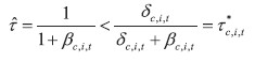 | (4) |
The difference is made by the contractionary effect of taxation on GDP.
5 The estimation method
In principle, the model parameters could be estimated separately for each country. However, due to the limited variation in tax rates over time, country-level estimates have low explanatory power. To better reflect general equilibrium effects and how a country’s economic structure shapes its Laffer curve, the parameters αc,i,t, δc,i,t and βc,i,t are modelled as functions of macroeconomic and policy variables.
To ensure that αc,i,t remains within the [0,1] interval, and thus that the tax to GDP ratio is always less than or equal to the tax rate, it is expressed using a logistic transformation:  | (5) |
where λ is a vector of parameters and Xc,i,t is the set of variables, discussed above.
The parameters βc,i,t and λc,i,t are similarly defined as exponential functions of the same set of explanatory variables: 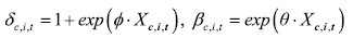 | (6) |
where θ and φ are vectors of parameters. This ensures that both the elasticity of the tax base and GDP to tax rate is negative.
The model is estimated in levels using a LASSO (Least Absolute Shrinkage and Selection Operator) technique. 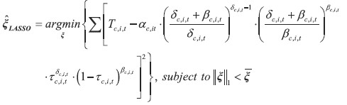 | (7) |
where αc,i,t =  , δc,i,t = 1+ exp( φ ⋅ Xc,i,t), βc,i,t = exp( θ⋅ Xc,i,t), and ξ = [ λ,φ,θ] T and all explanatory variables Χc,i,t are standardised prior to estimation.
The underlying functional relationship between tax rates and revenues is known and correctly specified, traditional estimators such as ordinary least squares or maximum likelihood are well suited and deliver efficient estimates. In the empirical estimation of Laffer curves, however, the functional form linking tax rates, tax bases, and revenues is inherently uncertain and non-linear. As shown in figure 1, the proposed model is flexible enough to incorporate several functional forms and yet sufficiently disciplined to incorporate the main theoretical properties of the Laffer curve 10.
Figure 2Examples of functional forms for different values of the parameters α, β, δ DISPLAY Figure
Moreover, allowing the parameters of the curve to depend on structural economic variables, improves robustness to misspecification and allows for cross-country heterogeneity in a way that traditional functional forms cannot. The use of a LASSO estimator helps prevent overfitting in complex, non-linear models by introducing a penalty term that reduces the variance of the estimates – at the cost of a small bias and reduces model misspecification bias. LASSO is particularly appropriate for forecasting and for identifying parsimonious representations of complex relationships when the true data-generating process is unknown.
Choosing the appropriate regularisation parameter is essential for the performance of the LASSO estimator. In this analysis, the optimal penalty value is selected through k-fold cross-validation. The full dataset contains 529 observations. In each cross-validation fold, 476 observations are used for training and 53 for validation. Since the model includes country fixed effects, the folds are stratified to ensure that each test set contains at least one observation per country. The optimal regularisation value is the one that minimises the Root Mean Squared Error (RMSE) across all test folds. The estimation method does not explicitly take into account the potentially distorting effects of the COVID-19 pandemic. The purpose of the long-term model is to estimate average structural relationships between tax rates and public revenues across a broad range of macroeconomic conditions. Excluding specific years would reduce the model’s ability to capture these long-term patterns and weaken its statistical precision. Moreover, removing or adjusting the pandemic years could introduce bias by arbitrarily excluding relevant observations. Any correction would rely on strong counterfactual assumptions, potentially distorting the estimated elasticities more than including the raw data. The use of regularised estimation techniques better mitigates the influence of extreme values by penalising overfitting. This ensures that unusually volatile observations in 2020-2021 do not unduly influence the estimated long-run parameters. The following quantifications are however made for the year 2019 to show the results in the last available year not affected by major economic shocks.
6 Estimation results
6.1 Personal income tax
The estimated parameters λ, Φ and θ allow us to draw the full Laffer curve for each country for all years, and to analyse which variables contribute more to the determination of each parameter. In 2019, according to the model’s estimates, 11 countries surpassed their revenue-maximising tax rate, τ*c,i,t, see table 4.
Table 4PIT, estimated effect of a 1 percentage point increase in the average tax wedge11 DISPLAY Table
The estimated Laffer curves for 2019 together with the observed value of revenues from personal income tax as a share of GDP for the same year are shown in figure 3.
Figure 3Personal income tax, the estimated Laffer curves by country, 2019 (% of GDP) DISPLAY Figure
A decomposition of the estimated effects in term of log differences is shown in figure 4. Countries such as Switzerland, Israel and Poland show the highest tax rate effects due to their relatively low rates, whereas Belgium, Germany and Italy exhibit the highest tax burden on personal income. Countries like Norway, Switzerland and Estonia experience the most significant GDP effects, indicating that an increase in the personal income tax rate would have a more severe negative impact on GDP in these countries. In contrast, Italy, Greece and France are least affected in this regard. Luxembourg, Ireland and Estonia display the largest tax base effects and Norway, Lithuania and Portugal the smallest.
Figure 4Personal income tax: decomposition of the effect of raising the average tax wedge by 1 percentage point on the tax revenue on GDP ratio DISPLAY Figure
6.2 Corporate income tax
The estimated parameters λ, φ and θ allow us to draw the full Laffer curve for each country for all years, and to analyse which variables contribute more to the determination of each parameter. In 2019, according to the model’s estimates, six countries surpassed their revenue-maximising tax rate, τ*c,i,t, see table 5.
Table 5CIT, estimated effect of a 1 percentage point increase in the tax rate12 DISPLAY Table
These effects though do not include the effects of tax competition among countries, exposed by the EU Tax Observatory ( 2004). The estimated Laffer curves for 2019 together with the observed value of revenues from corporate income tax as a share of GDP for the same year are shown in figure 5.
Figure 5Corporate income tax, the estimated Laffer curves by country (% of GDP) DISPLAY Figure
A decomposition of the estimated effects in terms of log differences is shown in figure 6. Countries such as Hungary, Ireland, and Lithuania show the highest tax rate effects due to their relatively low rates, whereas France, Portugal, and Germany exhibit the highest tax burden on corporate income. Countries like Hungary, Estonia, and Ireland experience the most significant GDP effects, indicating that an increase in the corporate income tax rate would have a more severe negative impact on GDP in these countries. In contrast, France, Italy, and Germany are least affected in this regard. Hungary, Latvia, and Lithuania display the largest tax base effects, while Luxembourg, Norway, and the Netherlands show the smallest effects.
Figure 6Corporate income tax, decomposition of the effect of raising the average tax wedge by 1 percentage point on the tax revenue on GDP ratio DISPLAY Figure
6.3 Value added tax
The estimated parameters λ, φ and θ allow us to draw the full Laffer curve for each country for all years, and to analyse which variables contribute more to the determination of each parameter. According to the estimated model only Norway and Hungary have already surpassed their revenue-maximising VAT rates, τ*c,i,t, in 2019 (see table 6).
Table 6VAT, estimated effect of a 1 percentage point increase in the average tax rate13 DISPLAY Table
The estimated Laffer curves for 2019 together with the observed value of revenues from value added tax as a share of GDP for the same year are shown in figure 7.
Figure 7Value added tax, the estimated Laffer curves by country (% of GDP) DISPLAY Figure
A decomposition of the estimated effects is shown in figure 8. Switzerland, Israel and United Kingdom exhibit the highest tax rate effects due to their low average VAT rates. On the other hand, Hungary, Finland, and Norway bear the highest VAT burdens. Belgium, Finland, and Ireland demonstrate the largest GDP effects, indicating that VAT rate increases would have a more pronounced negative impact on GDP in these countries. By contrast, Israel, Greece, and Portugal show the smallest GDP effects. The countries exhibiting the strongest tax base effects are Denmark, Switzerland, and the United Kingdom while Norway, Latvia, and Slovakia register the lowest tax base effect.
Figure 8Value added tax, decomposition of the effect of raising the average tax rate by 1 percentage point on the tax revenue on GDP ratio DISPLAY Figure
7 Comparison with alternative models
To evaluate the empirical performance of the proposed framework, the proposed model was estimated alongside several benchmark specifications commonly used in the Laffer-curve literature.
The proposed model systematically outperforms the alternative specifications in terms of out-of-sample fit (table 7).
Moreover, several benchmark specifications generate revenue schedules in which the tax-to-GDP ratio increases monotonically or continues rising beyond theoretically credible ranges (figure 9), whereas the proposed model, by construction, excludes such implausible configurations 14. The consequences are visible in table 7, which reports the estimated effect of a one-percentage-point increase in the corporate income tax rate for each model and country in the sample. The alternative specifications only predict positive increases in the revenue-to-GDP ratio, with relatively similar magnitudes across countries. In contrast, the proposed model yields more heterogeneous estimated effects, with several countries appearing to operate above their revenue-maximising tax rate 15.
Table 7CIT, Estimated effect of a 1 percentage point tax rate increase across models16 DISPLAY Table
Figure 9CIT, the estimated Laffer curves across models for selected countries (% of GDP) DISPLAY Figure
8 Conclusions
This paper proposes a parametric framework for estimating Laffer curves that combines theoretical discipline with the flexibility of machine learning techniques. The model is estimated using a LASSO technique, which enables the incorporation of a rich set of structural covariates while mitigating overfitting and reducing sensitivity to variable selection misspecification.
Consistently with the economic literature, the coefficients associated with the determinants of β – which captures the responsiveness of the tax base to tax rates – show that stronger governance and regulatory effectiveness are associated with lower estimated base elasticities, consistent with the interpretation that improved enforcement and compliance reduce the scope for avoidance and evasion. Conversely, variables capturing economic openness or sectoral composition are associated with higher estimated β in the case of corporate taxation, reflecting greater capital mobility or profit-shifting opportunities.
Similarly, the coefficients entering the specification of δ – which captures the responsiveness of GDP to tax changes – show how macroeconomic structure shapes the overall distortionary impact of taxation. The estimated effects of variables such as trade openness, sectoral shares, and labour market indicators suggest that economies with greater exposure to external competition or higher structural flexibility exhibit stronger output responses to tax rate changes.
The empirical results suggest that several OECD countries operate personal and corporate income tax rates above their estimated revenue-maximising levels. By contrast, most countries appear to remain below the revenue-maximising point for value-added tax, suggesting comparatively greater fiscal space in consumption taxation. The findings suggest that in several countries additional revenue mobilisation through higher income tax rates may be limited, whereas moderate adjustments in consumption taxation may yield revenue gains. More importantly, because the curvature of the Laffer relationship depends on structural characteristics, reforms aimed at strengthening institutions, reducing informality, broadening tax bases, and improving compliance may expand revenue capacity without increasing statutory rates.
Overall, the estimated effects of changes in tax rates are broadly consistent with estimates reported in previous empirical and quantitative studies. The present model, though, shows more heterogeneous results in the estimated revenue maximising tax rates. This is because the present framework derives them from the parameters β and δ, which capture the elasticities of the tax base and of the GDP based on economic, institutional and structural variables differently for each country.
In some cases, the estimated revenue-maximising rates are relatively high and substantially greater than the observed tax rates. This is the case for countries such as Czechia, Ireland, and Luxembourg for PIT, of Estonia, Hungary, and Ireland for CIT, and Finland, Ireland, and Luxembourg for VAT. This reflects a relatively high estimated responsiveness of GDP to the average tax rate (δ) together with a relatively low estimated responsiveness of the tax base (β). These results should be interpreted cautiously, as they are derived holding constant the independent variables that determine the estimated parameters α, β and δ. It is implausible to assume that substantial changes in tax rates would not affect these variables and, consequently, change both the shape of the curve and τ*c,i,t. Estimating the joint effects of tax increases on the dependent variables is beyond the scope of this paper. Moreover, the model does not account for international tax competition effects, which may become substantial in the case of large tax rate increases. However, for small increases in tax rates these effects can reasonably be considered negligible, and the proposed model provides a reliable estimate of the corresponding revenue impact. Similarly, the estimated value of τ*c,i,t should not be interpreted as a precise measure of how much tax rates can be increased, but rather as an indication of the proximity of current tax rates to their revenue-maximising level. At the same time, a different value of τ*c,i,t would imply a different degree of sensitivity of either the tax base or GDP to changes in the tax rate. These sensitivities are captured by the parameters β and δ, which in the model are estimated as functions of observable institutional, macroeconomic, and structural characteristics. Therefore, different values of τ*c,i,t should be mirrored by changes in the underlying institutional, macroeconomic, and structural conditions that shape these parameters. Accordingly, the framework is best interpreted as identifying structural revenue capacity conditional on prevailing institutional and macroeconomic conditions, rather than as prescribing immediate tax policy adjustments.
By enforcing the core theoretical properties of the Laffer curve and allowing its parameters to depend on observable structural characteristics, the proposed framework provides a flexible yet disciplined alternative to traditional reduced-form approaches. In settings where the true functional relationship between tax rates and revenues is unknown, regularisation plays a crucial role in stabilising estimation and reducing specification bias.
Relative to specifications commonly employed in empirical literature, the present framework differs in several respects. It imposes global theoretical consistency by construction. The estimated revenue effects of tax policy changes are more heterogeneous and can be decomposed into a mechanical rate effect, a tax-base effect, and a GDP effect. This heterogeneity is further explained by a set of indicators capturing institutional quality, economic structure, and demographic characteristics.
The framework developed in this paper provides policymakers a tool with which to assess revenue capacity in a manner that is both empirically robust and grounded in economic theory. In the context of rising fiscal pressures related to ageing, climate transition, and public investment needs, these estimates provide a structured benchmark for assessing feasible revenue mobilisation strategies. Future research could extend the framework to incorporate dynamic adjustment processes, international tax competition, or interactions between tax policy and tax administration reforms.
Appendix
DERIVATION OF THE MODEL
A similar approach can be adopted to identify the optimal average tax rate. Given an initial tax rate τ0 and total taxable income , B( τ0) an increase in the tax rate from τ0 to τ1 has two effects on tax revenues: a tax rate effect given by the increase in tax revenues at constant taxable income and a tax-base effect. As in the ETI model the latter can be assumed to be: 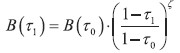 | (A1) |
where ζ is the elasticity of taxable income. Therefore, the total change in tax revenues can be written as: 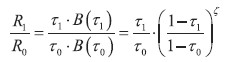 | (A2) |
Which in logarithms becomes:  | (A3) |
This can be expressed in differential terms as: 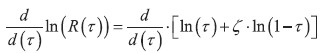 | (A4) |
Solving this equation one obtains:  | (A5) |
Where A is a scaling parameter and whose maximum is at:  | (A6) |
The model proposed is similar to equation (A5), where the scaling parameter A is replaced by a function of the average tax rate, which enforces the core properties of the Laffer curve and allows revenues to be expressed as a share of GDP instead of local currency units, as in most of the empirical cross-country literature:  Kt1-α Kt1-α | (A7) |
where τc,i,t is represents revenue item i, as a percentage of GDP. From equation A2, the change in tax revenues as a share of GDP can be written in the form: 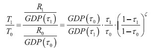 | (A8) |
While from equation (2), omitting the country-time indices, it can be written: 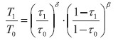 | (A9) |
Equating the two previous equations: 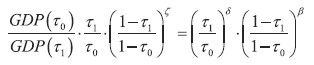 | (A10) |
If one assumes β = ζ. Then 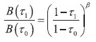 | (A11) |
and 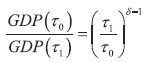 | (A12) |
Passing equation to logarithmic form and using equations A10 and A11, it is possible to decompose the change in tax revenues on GDP between two points in time τ0 and τ1 into the rate effect the tax-base effect and, the GDP effect in the following way. 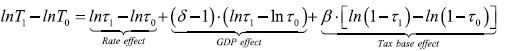 | (A13) |
Notes
* The author is grateful to two anonymous referees who have contributed to the quality of the final version of the paper.
1 OECD (2024), Tax wedge (indicator). doi: 10.1787/cea9eba3-en.
2 See, for example, Papp and Takáts (2008), Busato and Chiarini (2013) who analysed the effects of lowering tax rates on tax compliance; Feld and Frey (2002), Berenson (2018), who studied the effects of institutions and trust on implementation of tax policy; Sanyal, Gang and Goswami (2000), who modelled the effects of corruption on tax collections; Miravete, Seim and Thurk (2018), who studied how lack of market competition may flatten the Laffer curve.
3 See, for example, Heijman and van Ophem (2005).
4 See, for example, Trabandt and Uhlig (2011).
5 See, for example, Lozachmeur (2006), Cataldi, Kampelmann and Rycx (2011), Prammer (2019), who analysed the productivity-wage gap by age and how the effective tax rate changes with age; Creedy et al. (2010), Crowe et al. (2022), who quantified the effects of aging population on public revenue from income and consumption taxation.
6 See, for example, Akgun, Bartolini and Cournède (2017), who found a positive effect of inflation on public revenue from PIT and CIT; Kimbrough (2006), who estimated the revenue-maximising inflation rate.
7 See, for example, Holter, Krueger and Stepanchuk (2019).
8 See appendix for the derivation of the model from the ETI approach.
9 See appendix for the derivation of this decomposition.
10 For example, the quadratic form can be obtained from the proposed model with δ = 1, β = 1.
11 The estimated coefficients are not shown for reason of space, but the author would be happy to share regression results on request.
12 The estimated coefficients are not shown for reason of space, but the author would be happy to share regression results on request.
13 The estimated coefficients are not shown for reason of space, but the author would be happy to share regression results at the request.
14 Only 4 countries are shown for reason of space, but similar results are obtained for the other countries.
15 The table compares the results only for the CIT, but similar results are obtained for the PIT, and VAT.
* The author is grateful to two anonymous referees who have contributed to the quality of the final version of the paper.
1 OECD (2024), Tax wedge (indicator). doi: 10.1787/cea9eba3-en.
2 See, for example, Papp and Takáts ( 2008), Busato and Chiarini ( 2013) who analysed the effects of lowering tax rates on tax compliance; Feld and Frey ( 2002), Berenson ( 2018), who studied the effects of institutions and trust on implementation of tax policy; Sanyal, Gang and Goswami ( 2000), who modelled the effects of corruption on tax collections; Miravete, Seim and Thurk ( 2018), who studied how lack of market competition may flatten the Laffer curve.
3 See, for example, Heijman and van Ophem ( 2005).
4 See, for example, Trabandt and Uhlig ( 2011).
5 See, for example, Lozachmeur ( 2006), Cataldi, Kampelmann and Rycx ( 2011), Prammer ( 2019), who analysed the productivity-wage gap by age and how the effective tax rate changes with age; Creedy et al. ( 2010), Crowe et al. ( 2022), who quantified the effects of aging population on public revenue from income and consumption taxation.
6 See, for example, Akgun, Bartolini and Cournède ( 2017), who found a positive effect of inflation on public revenue from PIT and CIT; Kimbrough ( 2006), who estimated the revenue-maximising inflation rate.
7 See, for example, Holter, Krueger and Stepanchuk (2019).
8 See appendix for the derivation of the model from the ETI approach.
9 See appendix for the derivation of this decomposition.
10 For example, the quadratic form can be obtained from the proposed model with δ = 1, β = 1.
11 The estimated coefficients are not shown for reason of space, but the author would be happy to share regression results on request.
12 The estimated coefficients are not shown for reason of space, but the author would be happy to share regression results on request.
13 The estimated coefficients are not shown for reason of space, but the author would be happy to share regression results at the request.
14 Only 4 countries are shown for reason of space, but similar results are obtained for the other countries.
15 The table compares the results only for the CIT, but similar results are obtained for the PIT, and VAT.
Disclosure statement
The author has no conflicts of interest to declare.
References
Agell, J. and Persson, M., 2001. On the analytics of the dynamic Laffer curve. Journal of Monetary Economics, 48(2), pp. 397-414 [ CrossRef]
Agersnap, O. and Zidar, O., 2020. The Tax Elasticity of Capital Gains and Revenue-Maximizing Rates. NBER Working Paper, No. 27705 [ CrossRef]
Agha, A. and Haughton, J., 1996. Designing Vat Systems: Some Efficiency Considerations. The Review of Economics and Statistics, 78(2), pp. 303-308 [ CrossRef]
Akgun, O., Bartolini, D. and Cournède, B., 2017. The capacity of governments to raise taxes. OECD Economics Department Working Papers, No. 1407 [ CrossRef]
Berenson, M., 2018. Trust and Post-communist Policy Implementation. In: Taxes and Trust: From Coercion to Compliance in Poland, Russia and Ukraine. Cambridge University Press, pp. 12-55 [ CrossRef]
Bloch, D. [et al.], 2016. Trends in Public Finance: Insights from a New Detailed Dataset. OECD Economics Department Working Papers, No. 1345 [ CrossRef]
Busato, F. and Chiarini, B., 2013. Steady State Laffer Curve with the Underground Economy. Public Finance Review, 41(5), pp. 608-632 [ CrossRef]
Cataldi, A., Kampelmann, S. and Rycx, F., 2011. Productivity-Wage Gaps Among Age Groups: Does the ICT Environment Matter? De Economist, 159(2), pp. 193-221 [ CrossRef]
Creedy, J. [et al.], 2010. Population ageing and taxation in New Zealand. New Zealand Economic Papers, 44(2), pp. 137-158 [ CrossRef]
Crowe, D. [et al.], 2022. Population ageing and government revenue: Expected trends and policy considerations to boost revenue. OECD Economics Department Working Papers, No. 1737 [ CrossRef]
De Oliveira, F. G. and Costa, L., 2015. The VAT Laffer curve and the business cycle in the EU27: an empirical approach. Economic Issues, 20, pp. 29-44.
Diamond, P. and Saez, E., 2011. The Case for a Progressive Tax: From Basic Research to Policy Recommendation. Journal of Economic Perspectives, 25(4), pp. 165-190 [ CrossRef]
Feld, L. P. and Frey, B. S., 2002. Trust breeds trust: How taxpayers are treated. Economics of Governance, 3(2), pp. 87-99 [ CrossRef]
Feldstein, M., 1995. The Effect of Marginal Tax Rates on Taxable Income: A Panel Study of the 1986 Tax Reform Act. Journal of Political Economy, 103(3) [ CrossRef]
Ferreira‐Lopes, A., Martins, L. F. and Espanhol, R., 2019. The relationship between tax rates and tax revenues in eurozone member countries – exploring the Laffer curve. Bulletin of Economic Research, 72(2), pp. 121-145 [ CrossRef]
Heijman, W. J. M. and van Ophem, J. A. C., 2005. Willingness to pay tax: The Laffer curve revisited for 12 OECD countries. The Journal of Socio-Economics, 34(5), pp. 714-723 [ CrossRef]
Holter, H. A., Krueger, D. and Stepanchuk, S., 2019. How do tax progressivity and household heterogeneity affect Laffer curves? Quantitative Economics, 10(4), pp. 1317-1356 [ CrossRef]
Hsing, Y., 1996. Estimating the laffer curve and policy implications. Journal of Socio-Economics, 25(3), pp. 395-401 [ CrossRef]
Keen, M. [et al.], 1996. The Future of Value Added Tax in the European Union. Economic Policy, 11(23), pp. 373-420 [ CrossRef]
Kimbrough, K., P., 2006. Revenue maximizing inflation. Journal of Monetary Economics, 53(8), 1967-1978 [ CrossRef]
Liapis, K. J. [et al.], 2020. Investigating the relationship between tax revenues and tax ratios : an empirical research for selected OECD countries. International Journal of Economics and Business Administration, 8(1), pp. 215-229 [ CrossRef]
Lindsey, L. B., 1987. Individual taxpayer response to tax cuts: 1982–1984: with implications for the revenue maximizing tax rate. Journal of Public Economics [ CrossRef]
Lozachmeur, J. M., 2006. Optimal Age‐Specific Income Taxation. Journal of Public Economic Theory, 8(4), pp. 697-711 [ CrossRef]
Mankiw, N. G. and Weinzierl, M., 2006. Dynamic scoring: A back-of-the-envelope guide. Journal of Public Economics, 90(8-9), pp. 1415-1433 [ CrossRef]
Matthews, K., 2003. VAT evasion and VAT avoidance: Is there a European Laffer curve for VAT? International Review of Applied Economics, 17(1), pp. 105-114 [ CrossRef]
Miravete, E., Seim, K. and Thurk, J., 2018. Market Power and the Laffer Curve. Econometrica, 86(5), pp. 1651-1687 [ CrossRef]
Orsi, R., Raggi, D. and Turino, F., 2014. Size, trend, and policy implications of the underground economy. Review of Economic Dynamics, 17(3), pp. 417-436 [ CrossRef]
Papp, T. K. and Takáts, E., 2008. Tax Rate Cuts and Tax Compliance: The Laffer Curve Revisited. IMF Working Papers, WP/08/7 [ CrossRef]
Prammer, D., 2019. How does population ageing impact on personal income taxes and social security contributions? The Journal of the Economics of Ageing, 14, 100186 [ CrossRef]
Sanyal, A., Gang, I. N. and Goswami, O., 2000. Corruption, Tax Evasion and the Laffer Curve. Public Choice, 105(1/2), pp. 61-78 [ CrossRef]
Sanz-Sanz, J. F., 2016. The Laffer curve in schedular multi-rate income taxes with non-genuine allowances: An application to Spain. Economic Modelling, 55, pp. 42-56 [ CrossRef]
Trabandt, M. and Harald, 2011. The Laffer curve revisited. Journal of Monetary Economics, 58(4), pp. 305-327 [ CrossRef]
Tsuchiya, Y., 2016. Dynamic Laffer curves, population growth and public debt overhangs. International Review of Economics & Finance, 41, pp. 40-52 [ CrossRef]
|


