|
|
|
Abstract
In this paper, we discuss aggregate measures of marginal costs of public funds (MCF) in populations that are heterogeneous with respect to observed as well as unobserved characteristics. We first discuss how to compute MCF in selected examples of traditional (textbook) labour supply models. Next, we review two types of discrete labour supply models proposed in the literature. Subsequently, we discuss how to calculate aggregate measures of MCF for discrete labour supply models. Finally, we apply an estimated two-sector discrete labour supply model to compute MCF based on Norwegian data.
Keywords: marginal costs of public funds; discrete choice labour supply; compensated labour supply
JEL: J22, C25, H20, H40, H50
1 Introduction
Pigou (  1947 1947), Harberger ( 1964), and Browning ( 1976, 1987) introduced the concept of (compensated) marginal cost of public funds (MCF) as a measure of the cost of a marginal change in public revenue, defined as the reduction in consumers’ surplus relative to the increase in tax revenue. In the case of redistributing the revenue to the consumers as a lump-sum tax, the income effects of the tax change are neutralized, and the marginal cost of public funds relates only to the distortionary effect of the tax change. Subsequently, Mayshar ( 1900), Kleven and Kreiner ( 2006), and Jacobs ( 2018), have discussed how MCF can be obtained. Figari, Gandullia and Lezzi ( 2018) have discussed and calculated MCF for Italy, and Kleven and Kreiner ( 2006) have calculated MCF for five European countries (Denmark, France, Germany, Italy, and the UK). See Ballard and Fullerton ( 1992), Dahlby ( 2008), and Jacobs ( 2009) for reviews.
Nowadays, MCF is widely used in cost-benefit analysis. A well-known example where MCF is useful is in assessment of the toll price to finance a new road or bridge. It is important to stress that MCF is the marginal cost of taxation, given the existing tax system. It is not a tool adequate for evaluating tax reforms. Most of the previous works on MCF assume that a representative agent represents the behaviour of a population of individuals. However, this assumption is controversial. In fact, a representative agent does not exist unless very strong and unrealistic assumptions are met (Kirman, 1992; 2010). As shown in the critique of Kleven and Kreiner ( 2006), most works also ignore labour supply responses at the extensive margin.
Jacobs ( 2018) has proposed and discussed an aggregate measure of MCF based on a labour supply model in which utilities and wages depend on individual skills. In this paper, we propose an analogous aggregate measure of MCF. 1 In principle, one can use any empirical labour supply model to calculate MCF, if it accounts for observed and unobserved heterogeneity in preferences, such as the traditional textbook model. Unfortunately, the textbook labour supply model is highly stylized. Specifically, it ignores key features of the labour market, namely that workers have preferences over type of jobs and that the set of jobs that are available to a worker is limited. Furthermore, the textbook model ignores that the choice of hours of work is typically constrained, and often limited to full-time or part-time hours.
In recent years, many empirical analyses of labour supply have been based on the discrete choice framework (standard discrete labour supply model), pioneered by van Soest (ref8979#1995). The standard discrete labour supply model can easily accommodate non-linear and non-convex budget sets, which represents a major difficulty in the traditional model. It is therefore very convenient for use in empirical applications. However, an essential shortcoming of the standard discrete labour supply model is that it is, similarly to the traditional model, unable to deal with the restrictions mentioned above that workers face in the labour market.
A model that accounts for choice restrictions in the labour market is a modification of the standard discrete labour supply model, called the job choice model, proposed by Dagsvik ( 1994) and Dagsvik et al. ( 1988). For a review, see Dagsvik et al. ( 2014). Specifically, the job choice model is an extension of the standard discrete labour supply model that accounts for restrictions on workers’ choice sets of jobs. For example, due to institutional regulations and agreements between labour unions there are typically more jobs that offer full time and part time hours of work than jobs that offer other work schedules.
In the next section, we review briefly how previous measures of MCF have been defined and calculated based on the traditional textbook labour supply model for a representative agent (worker). In section 3, we discuss implementation of aggregate MCF in populations with heterogeneous workers. In section 4, we discuss the calculation of MCF for traditional labour supply models and in section 5 we review the discrete labour supply model and the job choice model, respectively. Section 6 discusses how MCF can be computed based on the standard discrete choice- and the job choice model, while section 7 reports the calculation of MCF for Norway based on the estimated two-sector job choice model.
2 Marginal cost of public funds based on the representative agent assumption
Consider the choice of labour supply of a representative agent and assume that the tax function is differentiable and convex, and can be represented by a scalar t. Let V (t, y) denote this indirect utility that corresponds to the direct utility of hours of work and let e (t, u) be the corresponding expenditure function, where u denotes utility. The indirect utility and the expenditure function depend on the tax system, the gross wage rate and (ex-ante) non-labour income y, but the gross wage rate is suppressed in the notation here. Moreover, let R (t, h, y) be the revenue collected by the government, as a function of the tax system, hours of work h and non-labour income y. Finally, let  denote the uncompensated labour supply function and denote the uncompensated labour supply function and  the corresponding compensated labour supply function. Håkonsen (1998), Ballard (1990), and Mayshar (1990), have proposed a measure of MCF given by the corresponding compensated labour supply function. Håkonsen (1998), Ballard (1990), and Mayshar (1990), have proposed a measure of MCF given by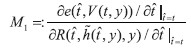 | (1) |
 represents any tax system and t represents the current (optimal) system. Jacobs (2018) argues that the definition above appears to suffer from an inconsistency because the numerator is a compensated measure, whereas the denominator is an uncompensated measure. Instead, one should replace the uncompensated labour supply function in the denominator by the compensated labour supply function. Thus, the modified measure that follows becomes represents any tax system and t represents the current (optimal) system. Jacobs (2018) argues that the definition above appears to suffer from an inconsistency because the numerator is a compensated measure, whereas the denominator is an uncompensated measure. Instead, one should replace the uncompensated labour supply function in the denominator by the compensated labour supply function. Thus, the modified measure that follows becomes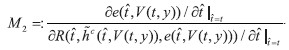 | (2) |
3 Marginal cost of funds in heterogeneous populations
In this section, we discuss an aggregate measure of MCF for heterogeneous populations that represents an extension of the measure proposed by Jacobs (2018).2
Consider a heterogeneous population of individuals who either work or do not work. Here, the possibility of unemployment is ruled out. The individuals are characterized by a vector of socio-economic variables x (say). Let V( t,y,x) denote the individual indirect utility as a function of a vector of individual characteristics x and let e( t,u,x) denote the corresponding expenditure function, given utility level u. Atkinson ( 1983) has proposed a welfare function that is analogous to the following function for ε ≠ 1 and equal to for ε = 1 where E is the expectation operator with respect to the population distribution of ( x,y) and ε is a parameter that reflects the inequality aversion of the government. However, in this paper, where the focus is on MCF, we need an aggregate money metric cost function, which is obtained by letting ε = 0. Note that when t =  ![]() ![]() then W( t) = Ey. Thus W( ) – Ey is the aggregate cost of replacing t by . If t is optimal then W( ) – Ey is always positive. Otherwise, W( ) – Ey might be negative if is better than t.
The actual tax system may be interpreted as optimally chosen by the authorities. This means that we assume the government has done its best to optimize taxes and redistribute income. We have no reasons to overturn the judgment of the politicians. We also assume that lump-sum taxes are not an alternative.
With ε = 0 it follows that  | (3) |
is the marginal aggregate cost associated with a marginal change of the actual (optimal) tax system t.
An obvious extension of the measures discussed in the previous section is 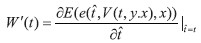 | (4) |
In a case in which the tax system is represented by a vector t, with components that are functionally dependent, one cannot use the measure in (4). Instead one can use the measure given by  | (5) |
where is “close” to t, and where and t now are vectors.
4 Traditional labour supply models
In empirical analysis and calculation of MCF one needs specifications of functional form expressions for the uncompensated and compensated labour supply and expenditure functions that are reasonably practical to work with. Below we shall briefly discuss two cases where explicit expressions can be obtained. For simplicity, we suppress the vector of individual characteristics in the notation.
4.1 Linear labour supply function
In this section, we consider the implementation of MCF in the case of the linear textbook labour supply functionwhere 1 – κ is the marginal tax rate (which is known) and w is the individual’s wage rate (Hausman, 1980, 1985). One or several of the parameters a, b and c may depend on individual characteristics to accommodate observed and unobserved heterogeneity in preferences. Note that the Slutsky conditions imply that the parameters a, b and c must satisfy specific inequalities. The expenditure function that corresponds to the linear supply function, as a function of the tax rate and utility level, is (Stern, 1986) 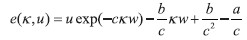 | (6) |
 | (7) |
If the tax function is non-linear, differentiable and convex, the labour supply function admits the form 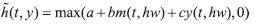 | (8) |
where m( t, hw) is the marginal wage rate at labour income hw and y( t, hw) is the so-called virtual non-labour income. Analogous expressions hold for the expenditure and the compensated labour supply functions. Thus, in this case the labour supply function is only given in implicit form because the right side of (8) depends on hours of work. However, it can still be estimated by known methods, either by using instrument variable techniques or by using the maximum likelihood method combined with the transformation of variables device and the corresponding Jacobian. In this case, it might be cumbersome to simulate M3 because one must solve non-linear equations for expenditure, uncompensated and compensated hours of work for each draw of the stochastic components.
4.2 Semi-log labour supply function
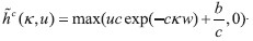
In this case, with a linear tax system, the uncompensated labour supply function has the form (Heckman, 1974) Also, in this case the Slutsky conditions imply restrictions on the parameters, a, b and c, see Stern (1986). The expenditure function of the wage rate and utility that corresponds to the semi-log supply function has the form (Stern, 1986)  | (9) |
5 Discrete labour supply models
As mentioned above, there are two types of labour supply models based on the discrete choice framework (McFadden, 1974) proposed in the literature. The standard discrete labour supply model was proposed by van Soest (1995) whereas Dagsvik (1994) and Dagsvik et al. (1988) proposed the job choice model, which contains the standard discrete labour supply model as a special case. For simplicity, we suppress the vector of individual characteristics in the notation also in this section.
5.1 The standard discrete labour supply model
The standard discrete labour supply model differs from the traditional textbook model in that the set of feasible hours of work is finite, say equal to D, and that the stochastic specification of the utility function differs from the traditional labour supply model.
An individual in the labour market faces the budget constraint| C(t,h,y) = hw + y − R(t,h,y) | (10) |
| U(h) = μ(C(t,h,y),h) + ε(h) | (11) |
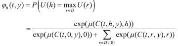 | (12) |
5.2 The job choice model
The job choice model allows the researcher to account for latent choice restrictions in the labour market. Such restrictions may explain why the distribution of hours of work typically show peaks at full-time and part-time hours of work and that some workers face smaller (latent) sets of job opportunities than other workers. In this model, the household derives utility from household consumption, leisure, and non-pecuniary latent job attributes.
Let k = 1, 2..., be an indexation of the jobs (latent) and let k = 0 represent no job. The utility function now has a slightly different form than the one given in (12), namely | U(h,k)=μ(C(t,h,y),h)+ε(k) | (13) |
where, as above, μ( C, h) is a positive deterministic function that is increasing in C and decreasing in h. Evidently, k = 0, if and only if h = 0. The taste shifters { ε( k)} are i. i. d. with standard Gumbel c. d. f. The taste shifters account for unobserved individual characteristics and unobserved job-specific attributes that affect preferences. The jobs have fixed job-specific hours of work schedules. Let B( h) be the set of jobs with hours of work h that are available to the agent. The sets B( h), h ∈ D, are individual-specific and latent. Moreover, let θ be the total number of jobs available (to the worker) and g( h) the proportion of jobs in B( h) with hours of work h. Thus, θ g( h) is the number of jobs with hours of work h in the set B( h). From (12) and (13) it follows that the probability that the agent will choose a specific job k in B( h) is given by the multinomial logit formula, namely Since the last expression does not depend on k the probability that the agent will choose any job with workload h follows by multiplying the probability above by the number of jobs θ g( h) in B( h), which yields 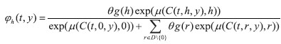 | (14) |
For h = 0, φ0 ( t,y) is obtained by replacing the numerator in (14) by exp( μ( C( t,0, y),0)). We note that (14) differs from (12) in that the exponential of the systematic parts of the utilities are weighted by the opportunity measure, { θ g(r)}.
The first econometric application of this type of modified logit model with latent “elemental” alternatives appears to be in Ben-Akiva and Watanatada ( 1981). They discuss both a discrete and a continuous version. Dagsvik et al. ( 1988) is the first published version of the job choice model applied to analyze labour supply behaviour. Formally, the utility maximization (with respect to hours of work) in the presence of these types of latent constraints can formally be viewed as an unconstrained maximization problem, namely the maximization of with respect to h where { ƞ( h)} are i. i. d. with standard Gumbel c. d. f. and where the structural part v is given by | v(C,h)=μ(C,h)+log(θg(h)) |
|
for h > 0 and v( C, 0) = μ ( C, 0) for h = 0. Thus, mathematically, the model given in (14) can be treated as if it were a standard discrete labour supply model with μ( C( t,h,y), h) replaced by v( C( t,h,y), h). Dagsvik and Jia ( 2016) have discussed identification of μ, θ and g( h) in the job choice model. They also provide a simplified version of the proof originally given by Dagsvik ( 1994) that the job choice model with discrete/continuous labour supply density follows from utility maximization (supplementary part of Dagsvik and Jia, 2016).
6 Marginal costs of public funds in the case of discrete labour supply models
For simplicity, we also drop the vector of individual characteristics in the notation in this section, but it is evident how the following analysis can be modified to account for observable individual characteristics. In the following, the notion “discrete labour supply model” is to be understood as either the standard discrete labour supply model or the job choice model. In the case of discrete labour supply models, one cannot use the standard approach discussed in section 3 because the utilities, compensated and uncompensated labour supply and expenditure functions are stochastic and cannot be expressed in closed form. Therefore, the usual approach does not apply. Instead, one can use an approach that is analogous to Dagsvik, Strøm and Locatelli (2021).
Define the operator Z+ by Z+ = max( Z, 0), and let yh(  ) be defined by
Consider a setting whereis any value of the tax parameter, different from t, and let  and and  |
|
Moreover, we assume the existence of a subsistence level of disposable income (minimum income necessary for survival) such that μ( x, h) = –∞ if disposable income is less than the subsistence level. Let a be a constant such that v( C( t, h, z), h) = –∞ when z ≤ – a. In the following, if ƒ( x1, x2,...) is a differentiable function of several variables we will use the notation ƒ( x1, x2,...) = ∂ƒ( x1, x2,...)/ ∂xj.
Theorem 1
Under the assumptions of the discrete labour supply model, we have that and The proof of Theorem 1 is given in appendix A.
Note that in Theorem 1 the tax system (represented by t) does not have to be a scalar, but can be any multidimensional vector. The results in Theorem 1 can be used to compute M4 given by the formula in (5).
Consider next the case where the tax function can be represented by a scalar t. This includes a tax system that can be expressed as tζ(y) where ζ(.) is a fixed function of taxable income, y (say).
Corollary 1
Assume that t is a scalar. Under the assumptions of the discrete labour supply model we have where The proof of Corollary 1 is given in appendix A.
Before stating the next result, we need to define right and left derivatives. Let ƒ( x) be a function of a real variable and define the right derivative of ƒ( x) by provided that the limit on the right side above exists. Similarly, define the left derivative of ƒ( x) by provided the limit on the right side above exists. If ∂ +ƒ(x)/∂x=∂ -ƒ(x)/∂x then ƒ( x) is differentiable. Let and define  and and  |
|
Under the assumptions of the discrete labour supply model we have, in a case in which t is a scalar, that and The proof of Corollary 2 is given in appendix A. From Corollary 2 we see that the marginal compensated effect ∂φhc ( t,y)/ ∂t does not exist unless the tax function is linear. Instead, one should use the right marginal compensated effect ∂+φhc ( t,y)/ ∂t in the case of a tax increase and the left marginal compensated effect ∂-φhc ( t,y)/ ∂t in the case of a tax decrease. In the present case, it is only relevant to deal with tax increases and one should therefore use the right marginal compensated effect. Regarding the intuition why the left and right marginal effects differ, see Dagsvik, Strøm and Locatelli ( 2021).
Corollary 3 Under the assumptions of the discrete labour supply model we have, in the case where t is a scalar, and The proof of Corollary 3 is given in appendix A.
Note that an implication of Corollary 3 is that which says that the marginal expected revenue can be computed by replacing Y( ) by y. The results of Corollaries 1 to 3 can be used to compute M3 given in (4).
7 Computation of MCF associated with an increase in minimum tax deduction
In this section, we discuss an evaluation of MCF that corresponds to a marginal increase in the minimum deduction level (below this level taxes on wage income are zero). This application is based on the sectoral job choice model (Dagsvik and Strøm, 2006). In the case of sectoral job choice there are several extensive margins, related to the choice of working or not and the choice of sector. There are two sectors, public and private. This model was estimated by using a sample of married women in Norway. Recall that the job choice model accommodates restrictions on the workers’ choice sets and thus enables us to rationalize observed peaks at full-time and part-time hours of work.
Like many countries, Norway has a progressive tax system for taxation of labour income, with stepwise linear parts. The actual structure of the tax system in 1994 is given in appendix B. In general, whenever a tax rate is changed in a piecewise linear tax system one must also change other tax rates too, since the tax function is continuous. This is not necessary when the minimum deduction level is changed. Thus, in this application the tax parameter t is a scalar, equal to the minimum deduction level.
Our estimate of the marginal cost of public funds, given in equation (4), is 1.15, which is in the lower part of the range that others have found, also for Norway. Numerous studies have demonstrated that married women respond more strongly to changes in economic incentives than single women and men, married or not. Since we include only married women in our sample, our estimate is, most likely, higher than if men and single women had been included in the sample. Thus, if the whole population had been used in the calculation of MCF, most likely the estimate of the marginal cost of funds in Norway would have been less than 1.15.
8 Conclusion
In this paper, we have discussed aggregate measures of MCF, which account for observed as well as unobserved population heterogeneity in preferences, with special reference to discrete labour supply models. In the context of the discrete labour supply model, which are based on a stochastic formulation of primitives, one cannot use the usual approach to calculate MCF because the uncompensated as well as the compensated labour supply and the expenditure functions are stochastic and cannot be expressed in closed form. We have therefore used an alternative approach that enables the calculation of aggregate measures of MCF in the case of discrete labour supply models. Finally, we have used an estimated version of the job choice model to compute the MCF of the Norwegian income tax system that corresponds to a marginal change of the minimum deduction level.
Appendix A
Recall that yh ( ) is defined by ) is defined by  where is any tax parameter different from where is any tax parameter different from  and and  v(C(t,h,y),h)). For simplicity we use the notation dz = (z + dz, z). v(C(t,h,y),h)). For simplicity we use the notation dz = (z + dz, z).
Lemma A1
Suppose Z is a non-negative random variable with c. d. f. F( z) where F( z)= 0 when z ≤ –a where a is a constant. Then The result of Lemma A1 follows by integration by parts.
Lemma A2 Under the assumptions of the discrete labour supply model we have that Lemma A3 Under the assumptions of the discrete labour supply model we have that and Lemmas A2 and A3 are applications to the i. i. d. Gumbel case of Theorems 3 and 4 of Dagsvik and Karlström ( 2005). In fact, Lemma A3 corrects Theorem 4 of Dagsvik and Karlström ( 2005), as the latter claims that which in general is not true as it is not always the case that for all x in D.
Lemma A4 Under the assumptions of the discrete labour supply model the ex post compensated choice probability of working h hours is given by The result Lemma A4 follows immediately from Lemma A3.
Q. E. D.
Proof of Theorem 1: The first relation in Theorem 1 follows immediately from Lemmas A1 and A2. The second relation in Theorem 1 follows from Lemma A3.
Q. E. D.
Proof of Corollary 1: Assume first that  ![]() and that  is small. It follows that   | (A1) |
We have Using the last relation and the mean value theorem for integrals, we obtain that the following:  | (A2) |
where z*∈( yx ( ), y). When → t it follows that z* → y. Hence, so that (A.2) implies that  | (A3)
|
When yh( ) < y a similar argument as above leads to the same result as in (A.3). By implicit differentiation we obtain implying that  | (A4) |
Hence, by Lemma A1, (A.1), (A.3) and (A.4) it follows that which implies the result in Corollary 1.
Q. E. D.
Proof of Corollary 2: When - t=Δ t is small it follows from Lemma 3 that 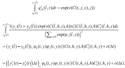 | (A5) |
When Δ t > 0, then  | (A6) |
and when Δ t < 0, then 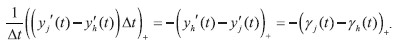 | (A7) |
Hence, (A.6) implies that when Δ t > 0 then 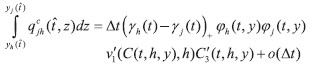 | (A8) |
whereas when Δ t < 0 (A.7) yields 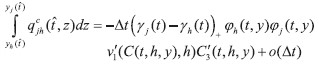 | (A9) |
Furthermore, 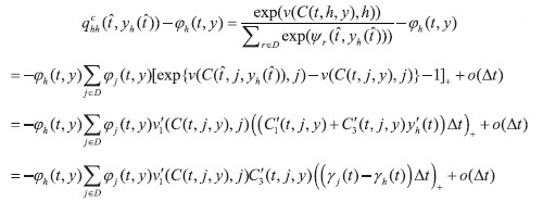 | (A10) |
Hence, when Δ t > 0 (A.10) implies that  | (A11) |
whereas when Δ t < 0 then  | (A12) |
The result of Corollary 2 now follows from (A.8) and (A.11), and (A.9) and (A.12), respectively.
Q. E. D.
Proof of Corollary 3:
Note first that by the mean value theorem for integrals there exists a number,  such that  | (A13) |
because  , when Δ t → 0 so that  tends towards zero when Δ t → 0 Suppose next that Δ t > 0. By using (A.13) and Lemma A4 we get that which leads to the first relation of the corollary. The case in which Δ t < 0 is proved in a similar way and implies the second relation of the corollary.
Q. E. D.
Appendix B
TAX FUNCTIONS
The tax functions for married couples are piecewise linear and given in the tables below. The minimum deduction level t referred to in the text equals NOK 41,907 for a married non-working woman and NOK 20,954 for a working woman.
Table B1Tax function in 1994 for a married non-working woman whose husband is working, 1994 DISPLAY Table Table B2Tax function in 1994 for a married working woman NOK 1994 DISPLAY Table
Funding
This study was funded by the Ragnar Frisch Centre of Economic Research, Oslo,
Norway, and by small research grants from the Department of Economics, University of Oslo.
Notes
* We are grateful for comments by Terje Skjerpen and two anonymous referees. We also thank Marilena Locatelli for her assistance.
1 Some of the results in this paper were also obtained in Dagsvik, Strøm and Locatelli (2014).
2 For a recent discussion of applying aggregate money metrics in welfare analysis, see Bosmans, Decancq and Ooghe (2018).
3 In the traditional case utility is assumed to be quasi-concave to ensure a unique maximum. In the discrete
case with finite D this assumption is no longer needed.
* We are grateful for comments by Terje Skjerpen and two anonymous referees. We also thank Marilena Locatelli for her assistance.
1 Some of the results in this paper were also obtained in Dagsvik, Strøm and Locatelli ( 2014).
2 For a recent discussion of applying aggregate money metrics in welfare analysis, see Bosmans, Decancq and Ooghe ( 2018).
3 In the traditional case utility is assumed to be quasi-concave to ensure a unique maximum. In the discrete
case with finite D this assumption is no longer needed.
Disclosure statement
John K. Dagsvik has received research grants from the Ragnar Frisch Centre of
Economic Research, Oslo, Norway. Steinar Strøm has received research grants
from the Ragnar Frisch Centre of Economic Research, Oslo, Norway. The authors
declare that they have no conflict of interest.
References
Atkinson, A. B., 1983. The Economics of Inequality. Oxford, UK: Clarendon Press.
Ballard, C. L. and Fullerton, D., 1992. Distortionary Taxes and the Provision of Public Goods. Journal of Economic Perspectives, 6(3), pp. 117-131 [ CrossRef]
Ballard, C. L., 1990. Marginal Welfare Cost Calculations: Differential Analysis vs. Balanced-Budget Analysis. Journal of Public Economics, 41(2), pp. 263-276 [ CrossRef]
Ben-Akiva, M. and Watanatada, T., 1981. Application of a Continuous Spatial Choice Logit Model. In: C. Manski and D. McFadden, eds. Structural Analysis of Discrete Data. Washington: MIT Press, pp. 320-341.
Browning, E. K., 1976. The Marginal Cost of Public Funds. Journal of Political Economy, 84(2), pp. 283-298 [ CrossRef]
Browning, E. K., 1987. On the Marginal Welfare Cost of Taxation. American Economic Review, 77, pp. 11-23.
Dagsvik, J. K. [et al.], 1988. The Impact on Labor Supply of a Shorter Workday: A Micro-econometric Discrete/Continuous Choice Approach. In: R. A. Hart, ed. Employment, Unemployment and Labor Utilization. Winchester, MA: Unwin Hyman, Inc.
Dagsvik, J. K. [et al.], 2014. Theoretical and Practical Arguments for Modeling Labor Supply as a Choice among Latent Jobs. Journal of Economic Surveys, 28(1), pp. 131-151 [ CrossRef]
Dagsvik, J. K. and Jia, Z., 2016. Labor Supply as a Choice among Latent Jobs: Unobserved Heterogeneity and Identification. Journal of Applied Econometrics, 31(3), pp. 487-506 [ CrossRef]
Dagsvik, J. K. and Karlström, A., 2005. Compensating Variation and Hicksian Choice Probabilities in Random Utility Models that are Nonlinear in Income. Review of Economic Studies, 72(1), pp. 57-76 [ CrossRef]
Dagsvik, J. K. and Strøm, S., 2006. Sectoral Labor Supply, Choice Restrictions and Functional Form. Journal of Applied Econometrics, 21(6), pp. 803-826 [ CrossRef]
Dagsvik, J. K., 1994. Discrete and Continuous Choice, Max-Stable Processes, and Independence from Irrelevant Attributes. Econometrica, 62(5), pp. 1179-1205 [ CrossRef]
Dagsvik, J. K., Strøm, S. and Locatelli, M., 2019. Marginal Compensated Effects in Discrete Labor Supply Models. CESifo, No 7493 [ CrossRef]
Dagsvik, J. K., Strøm, S. and Locatelli, M., 2021. Marginal Compensated Effects in Discrete Labor Supply Models. Journal of Choice Modelling, 41 [ CrossRef]
Dahlby, B., 2008. The Marginal Cost of Public Funds: Theory and Applications. Cambridge, MA: MIT Press [ CrossRef]
Figari, F. L., Gandullia, L. and Lezzi, E., 2018. Marginal Cost of Public Funds: From the Theory to the Empirical Application for the Evaluation of the Efficiency of the Tax-Benefit Systems. The B.E. Journal of Economic Analysis & Policy, 18(4), pp. 1-16 [ CrossRef]
Håkonsen, L., 1998. An Investigation into Alternative Representations of the Marginal Cost of Public Funds. International Tax and Public Finance, 5, pp. 329-343 [ CrossRef]
Harberger, A. C., 1964. The Measurement of Waste. American Economic Review, 54, pp. 58-76.
Hausman, J. A., 1980. The Effects of Wages, Taxes and Fixed Costs on Women’s Labor Force Participation. Journal of Public Economics, 14(2), pp. 161-192 [ CrossRef]
Hausman, J. A., 1985. The Econometrics of Non-linear Budget Sets. Econometrica, 53(6), pp. 1255-1282 [ CrossRef]
Heckman, J. J., 1974. Shadow Prices, Market Wages and Labor Supply. Econometrica, 42(4), pp. 679-694 [ CrossRef]
Jacobs, B., 2009. The Marginal Cost of Public Funds and Optimal Second-Best Policy Rules. Mimeo. Rotterdam: Erasmus University Rotterdam.
Jacobs, B., 2018. The Marginal Cost of Public Funds is One at the Optimal Tax System. International Tax and Public Finance, 25, pp. 883-912 [ CrossRef]
Kirman, A., 1992. Whom or what does the Representative Agent Represent? Journal of Economic Perspectives, 6(2), pp. 117-136 [ CrossRef]
Kirman, A., 2010. The Economic Crisis is a Crisis for Economic Theory. CESifo Economic Studies, 56(4), pp. 498-535 [ CrossRef]
Kleven, H. J. and Kreiner, C. T., 2006. The Marginal Cost of Public Funds: Hours of Work versus Labor Force Participation. Journal of Public Economics, 90(10-11), pp. 1955-1973 [ CrossRef]
Mayshar, J., 1990. On Measures of Excess Burden and Their Application. Journal of Public Economics, 43(3), pp. 263-289 [ CrossRef]
McFadden, D., 1974. Conditional Logit Analysis of Qualitative Choice Behavior. In: P. Zarembka, ed. Frontiers in Econometrics. New York: Academic Press, pp. 105-142.
Pigou, A. C., 1947. A Study in Public Finance. London: Macmillan.
Stern, N., 1986. On the Specification of Labour Supply Functions. In: R. Blundell and I. Walker, eds. Unemployment, Search and Labour Supply. London: Cambridge University Press, pp. 143-189.
Van Soest, A., 1995. A Structural Model of Family Labor Supply: A Discrete Choice Approach. Journal of Human Resources, 30(1), pp. 63-88 [ CrossRef]
|


